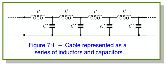
Cables are generally analysed as a form of Transmission Line. The E-fields between the conductors mean that each length of the pair of conductors has a capacitance. The H-fields surrounding them mean they also have inductance. The longer the cable, the larger the resulting values of these might be. To allow for this variation with the length, and also take into account the fact that signals need a finite time to pass along a cable, they are modelled in terms of a given value of capacitance and inductance ‘per unit length’. A run of cable is then treated as being a series of incremental (i.e. small)  elements chained together as shown in figure 7·1. (Note that I have identified these as
  and
and  and use the primes to indicate that they are values-per-unit-length.)
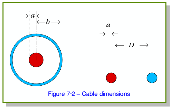
The amount of capacitance/metre and inductance/metre depends mainly upon the size and shape of the conductors. The inductance relates the amount of energy stored in the magnetic field around the cable to the current level. The capacitance relates the amount of energy stored in the electric field to the potential difference between the conductors. For co-ax and twin feeders the values are given by the expressions in the table below, where the relevant dimensions are as indicated in figure 7·2.
|
| Capacitance F/m
| Inductance H/m
| Impedance 
|
| Co-axial cable
|

|

|
|
| Twin Feeder
|

|

|
|
Note that when  we can say that
  . Since we require the wires not to touch, this condition will alway be true for a twin feeder, so we can use an alternative form for the above expressions. Some textbooks assume that
  and since when this is the case,
  , they then give a simplified set of expressions for the properties of a twin feed where the above
  terms are replaced with
  .
.
For cables of the kinds considered here, we can make a few general comments which apply whatever their detailed shapes, sizes, etc.
The Characteristic Impedance depends upon the ratio of the values of the capacitance per metre and inductance per metre. To understand its meaning, consider a very long run of cable that stretches away towards infinity from a signal source. The source transmits signals down the cable which vanish off into the distance. In order to carry energy, the signal must have both a non-zero current, and a non-zero potential. (i.e. both the E-field and the H-field must exist and propagate along, guided by the cable.) Since the far end is a long way away, the signals transmitted from the source can’t initially be influence by the properties of any destination before they finally arrive. Hence the  ratio of the field carried along the cable (and hence the current/voltage ratio) are determined solely by properties of the cable. The result, when the signal power vanishes, never to be seen again, is that the cable behaves like a resistive load of an effective resistance set by the cable itself. This value is called the Characteristic Impedance,
  , of the cable. In general, for a loss-free cable, its value is given by
and the velocity with which the signal (and hence its energy) propagate along the cable is given by
which, if we assume no magnetic materials is involved, will be equivalent to a velocity of
where  represents the relative permittivity of the insulating (dielectric) materials in which the conductors are nominally embedded.
As a matter of convention, there is a tendency for many co-axial cables to be designed and manufactured to have an impedance of either 75  (used by TV and VHF radio manufacturers) or 50
  (used by scientists and engineers for instrumentation and communications). Engineers use a variety of type and impedances of cables. At RF, the use of 300
  twin feed is fairly common, and 600
  is often used at audio frequencies. Standard values tend to be adopted for convenience in a given application area as this makes it easier for people to build systems from compatible elements.