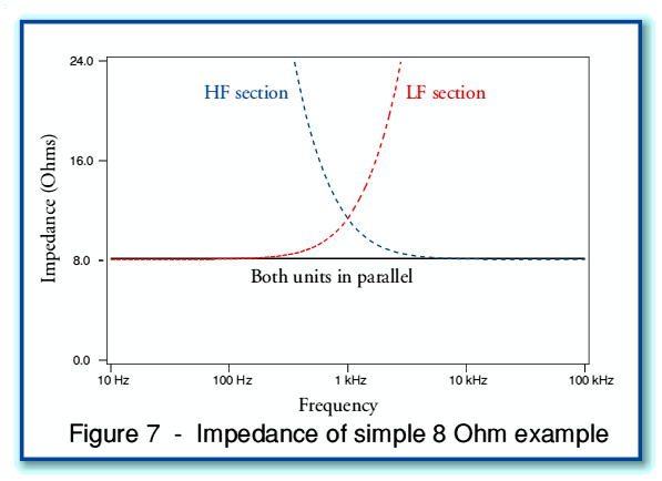
To assess the implications of the model of bi-wiring we have produced we can now examine the results of choosing some example values. For simplicity, the following assumes that the nominal impedance of the loudspeaker units is such that  , and that the nominal cross-over frequency is
  kHz. Figure 7 shows the input impedance of the resulting loudspeaker system as a function of frequency. Note that the frequency scale is logarithmic, and that in each case it is the magnitude (modulus) of the impedance that is plotted as a function of frequency.
Figure 7 and the graphs that follow have been plotted from numerical results obtained from some simple C++ programs. The results shown in Fig 7 confirm that our simple model has the property that the impedance of the LF and HF sections when used connected in parallel is equal to  at all frequencies. This may be understood in terms of regarding the variations in impedance of the LF and HF sections cancelling out.
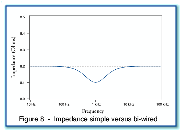
Let us now consider using an amplifier whose output impedance is 0·1 Ohms, and cables whose series resistance is 0·1 Ohms. For simplicity, we ignore cable inductance and assume that the cable is essentially purely resistive. We can now compare the results of using a single cable of this type (arrangement as shown in Fig 5) with using a pair of identical cables (arrangement as Fig 6). Figure 8 shows the how the total impedance seen by the amplifier varies with frequency in each case.
The broken black line in Figure 8 shows the impedance seen by the amplifier when using a single wire. Since this means the HF and LF units are connected together in parallel at the speaker end of the cable, the speaker looks like an 8 Ohm load at all frequencies. The signal voltages being generated by the amplifier see this impedance through the series impedance of the amplifier output and cable, thus in this case producing a total impedance of 8·2 Ohms at all frequencies.
The solid blue line in Figure 8 shows the impedance seen by the amplifier when bi-wiring is employed. In this case an independent 0·1 Ohms of cable impedance is seen in series with the HF and LF sections. The parallel combination is then seen in series with the amplifier’s output impedance. The bi-wiring arrangement can be seen to modify the impedance of the system as seen by the amplifier in a frequency dependent manner. The chosen cross-over frequency for this example was 1 kHz. Looking at Figure 8 it can be seen that changing from using a single cable to a bi-wiring arrangement caused a change in overall impedance which is most noticeable at this frequency. In this case it can be seen that at 1 kHz the total impedance of the system seen by the amplifier is 0·1 Ohms lower when bi-wired than when a single cable is employed. This change may be regarded as a consequence of the separate cable impedances altering the effective roll-over frequencies of the HF and LF sections so that they are no longer identical. The result is that the system’s impedance value is no longer constant over the whole frequency range.
The above result is an interesting one as it implies that bi-wiring may change the impedance properties of the total load system seen by the amplifier. If the sound power produced depends upon the square of the current fed to the system, this implies that the frequency response may perhaps be changed by bi-wiring as a result of interactions between the choice of cabling arrangement and the input impedances/networks of the loudspeaker units.
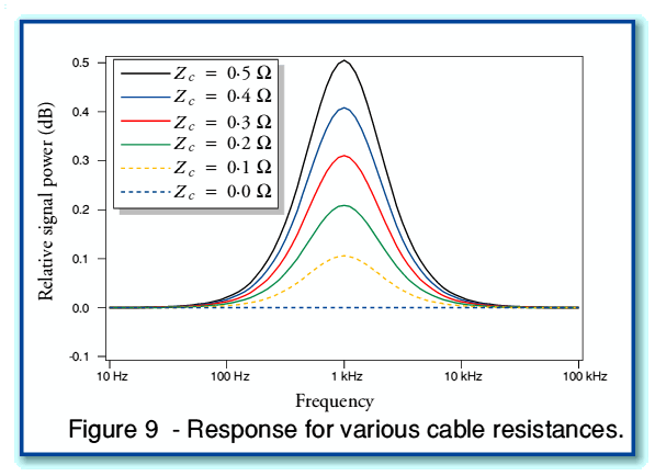
Figure 9 illustrates some examples of the changes in frequency response which the alterations in system impedance imply may produce. The curves are for a series of different choices of cable series resistance/impedance,  . In each case the amplifier output impedance is assumed to be 0·1 Ohms. Hence we can use this set of plots to get an impression of how the behaviour may vary if we change the cable resistance but use the same amplifier and speaker in each case. Looking at the plots we can see that for these specific examples we happen to get a variation in signal level at the crossover frequency which, in decibels, is approximately the same as the chosen cable series resistance in Ohms.
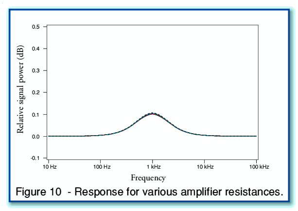
Figure 10 shows what happens if we keep the cable resistances fixed at 0·1 Ohms, and vary the output impedance of the amplifier. As with Figure 9, a set of curves are plotted, but in this case for  0, 0·1, 0·2, 0·3, 0·4, and 0·5 Ohms. Looking at Figure 10, we can see that all these plots are very similar. Indeed, they are so close together on the graph that it is not obvious how many curves are plotted. Considering Figures 9 and 10 taken together, leads to the implication that – in terms of comparing bi-wiring with using a single cable – changing the cable resistance may have an effect, but that varying the amplifier’s output resistance has little or no effect.
The above results imply that bi-wiring may alter the frequency response and that, when using a very simple speaker system with an impedance of around 8 Ohms, this variation may be of the order of 0·1 dB when using cables whose series resistance is around 0·1 Ohms. Thus, in principle, it seems possible that bi-wiring may alter the system’s frequency response. The details of any change will then depend upon the series impedance of the cables, and the impedance properties of the loudspeaker.
Two things should be kept in mind, however:
- In general many loudspeaker cables will have a series resistance value well below 0·1 Ohms. Indeed, a low value is advisable to avoid other types of interaction with the loudspeaker input impedance. Thus in practice the actual variations may well be much smaller than those plotted in Figure 9. As a result, it is debatable if any variations in practice will normally be large enough to be audible or to be regarded as being of any real consequence. Moving your head a few centimetres when listening may have a larger effect in many rooms.
- The model used here is a very simple one. Hence we should really only consider these results as implying that effects can occur in principle. The plots should not be taken to indicate what will actually happen with a more complex and realistic system.
It is also worth bearing in mind that the detailed analysis carried out here assume coherent addition of the HF and LF signals. This will be correct for a a listener at a fixed point when considering direct radiation from the loudspeaker system. The situation when the diffuse soundfield of the loudspeaker is taken into account may be more complex. However for this analysis we are simply interested in an “in principle” answer. Hence we can see this as another complication which means the actual performance in reality may well differ from the above results, but that a small change due to bi-wiring remains possible.
Thus we can conclude that there may be a small effect due to bi-wiring, but the above tends to imply it may normally be so small as to have little significance. In order to say more, a detailed model of specific realistic systems, and/or some precise measurements, would be required. These might reveal a more noticeable effect in some cases, but the above taken by itself implies the effects will usually be very small if low series impedance cables are used. It is also perhaps worth bearing in mind that - even in a case where any change in frequency response is large enough to be audible - this does not establish that the bi-wired arrangement will inevitably then be “better” than using a single cable. That would depend upon the circumstances of use, and the preferences of the listener.