One of the arguments presented in the web forum thread I’ve already examined on a previous webpage is that there is a difference between a bi-wired speaker system and conventional wiring due to a difference in their cable power dissipation behaviours. So let’s examine the systems described in the thread and see what difference there may be between them in practice. Consider this as a detective story...
The Mystery of the Cable Conundrum
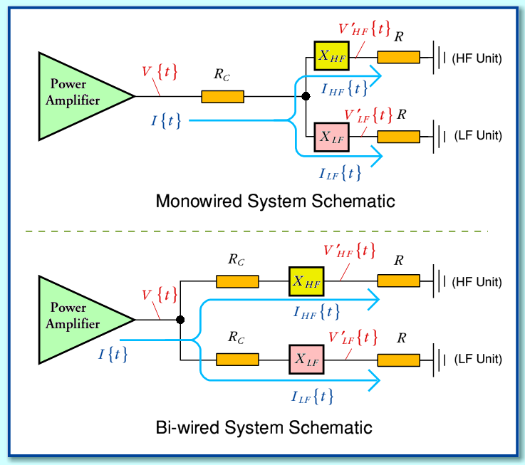
We can represent the conventional (‘monowired’) and ‘bi-wired’ systems by the arrangements shown in the above diagram. The loudspeaker is assumed to consist of a an HF unit (‘tweeter’) and LF unit (‘woofer’) which are intended to deal with distinct frequency bands. For the sake of simplicity we can assume each of these units behaves, electrically, like a resistive load, and give them the same resistance value,  .
.
The loudspeaker is assumed to operate with the HF unit dealing with all frequency components in the signal above a chosen frequency, and the LF unit dealing with all frequency components below this frequency. This means we have to place appropriate networks or filters in between each unit and the input signal to ensure they are only presented with signal components in the desired frequency range. Ideally the filters should not lose any of the intended signal, but should also completely block any frequencies which are not in the band which the unit is intended to handle.
In order to ensure this, we have to employ a pair of networks which have frequency-dependent properties. These are represented in the above diagrams by the items labelled with  and
and  .
.
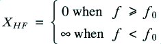
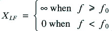
We can then define the required behaviour of these networks by saying that
and
where  is an appropriate value for the frequency which represents the boundary between the high and low frequency bands which we wish to direct to the HF and LF units respectively. The above definitions mean that the
  filters act like direct links in the desired frequency bands, but like open circuits outside that band. This ensures no ‘leakage’ of current or power into the ‘wrong’ unit.
In practice the networks employed in a real loudspeaker can only approach the above ‘ideal’ behaviour. This means they will generally have a non-zero series impedance in the frequency range they are designed to pass, and a finite impedance in the band they are designed to stop (block). That situation, with an example of a simple choice of a real pair of networks, has been examined on other webpages. So here I will examine this ‘ideal’ case where the networks behave as defined above...
The Signals
For the sake of example, let’s assume the signal emerging from the amplifier has the voltage pattern
where the frequencies are chosen so that  and
and  .
.
In both the monowired and bi-wired arrangements the HF component will behave as if  and
and  . Similarly, the LF component will behave as if
  and
and  . This ensures that each loudspeaker unit will only have frequency components in the relevant frequency range applied to it.
i.e. we can say that
and
To simplify the following expressions we can define
This lets us re-write the above as
and
Note that these voltages are not necessarily what we would observe on the actual terminals of a bi-wirable loudspeaker system. The primes are to warn us that the voltages referred to above are the values on the ‘other side’ of the filter networks, inside the loudspeaker.
These voltage will produce currents of
and
through the HF and LF units of the loudspeaker.
The rate of energy flow (i.e. power) from the amplifier into either system will be
The power delivered into each of the speaker units will be
and
It is worth noting that the above values remain the same, regardless of whether the system is monowired or bi-wired. i.e. The power required from the amplifier, and the powers delivered to into the units remain the same for both arrangements. So in practice they would actually deliver identical results. On that basis, no difference could be audible, and so there would be no real point in choosing bi-wiring over monowiring. But are the systems actually identical?...
The Conundrum
Clearly, the systems cannot be the same in every respect because they are physically different arrangements. However the above shows that – in terms of the amplifier output and the signal levels at the speaker units – the two arrangements being considered behave in exactly the same way. So where are the differences, and how do they arise?
One distinction between the two arrangements has been described in the web forum thread. This addresses the levels of power dissipation in the connecting cables. It is then argued that this means that the arrangements will not perform in the same way in use. Let’s therefore examine the cable dissipation levels for the two systems.
For the monowired case the power dissipation in the cable resistance will be
For the bi-wired system we have two cable dissipations, for the HF and LF cables which will be
with the total cable dissipation for the bi-wired case therefore being
It is immediately obvious that – as pointed out in the web thread – the levels of cable dissipation are not identical.
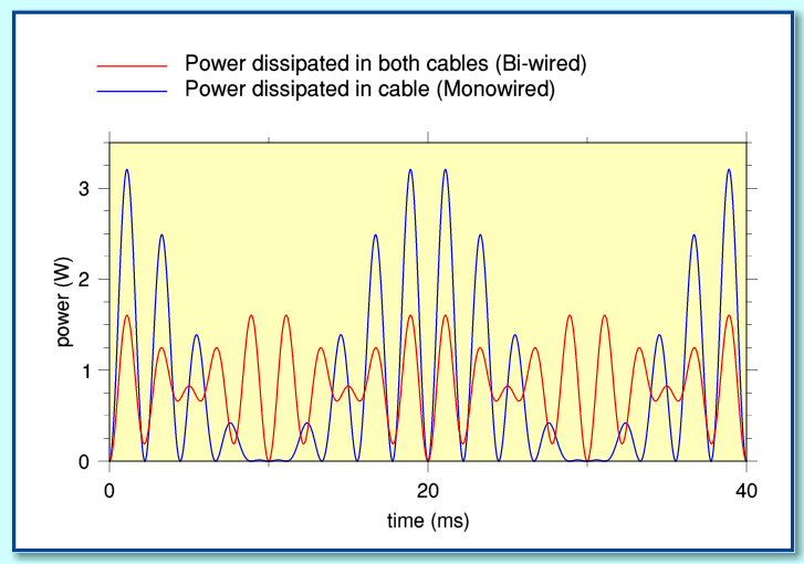
For the sake of illustration we can use the same example as employed on the previous webpage. This is a waveform with two sinusoids. Both having a peak voltage of 10V at the amplifier output, and with frequencies of 200 Hz and 250 Hz. It is assumed that  Hz so that one of these components goes to the HF unit and the other to the LF unit. The cables are assumed to have a resistance of 1 Ohm, and the loads assumed to be 10 Ohms.
Note that these values are arbitrary. I could have chosen two other frequencies. Provided that one were above  and the other below
  the conclusions would have been the same.
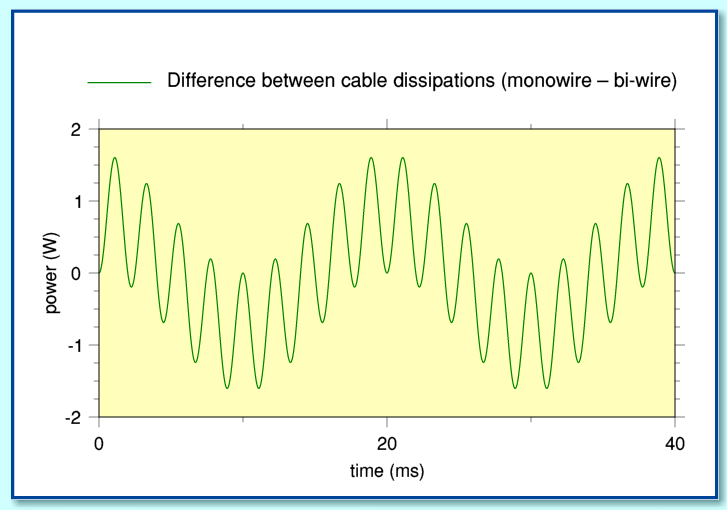
Using these values we can plot the above graphs showing how the resulting cable dissipations vary with time for the monowired and bi-wired arrangements. The shapes are clearly different, confirming that the patterns of dissipation are not identical.
If we subtract total the cable dissipation in the bi-wired arrangement from that in the monowired arrangement we can define this difference to be
which, using the example of a signal with an HF and a LF sinusoid as above becomes
Using the same example as above we can plot a graph like that shown below.
This displays the difference between the cable dissipations for the two arrangements when they are driven by the same test waveform.
The above results do seem to present us with an anomaly or paradox, as described in the web thread. The signal power level and current injected into the system by the amplifier is identical in both arrangements. Each speaker unit has the same power, current, and voltage delivered to it with both arrangements. Yet the cable loss patterns are different! The monowired case shows a ‘cross product’ term involving both signal frequencies which is absent when the system is bi-wired. Does this not mean that the monowired system has a problem which is avoided by bi-wiring?
The Missing Link(s)
To resolve the above conundrum let us now turn our attention to the items we haven’t yet examined in detail. What is happening to the filter networks,  , and
, and  ? These are – so far – the ‘missing links’ in the argument.
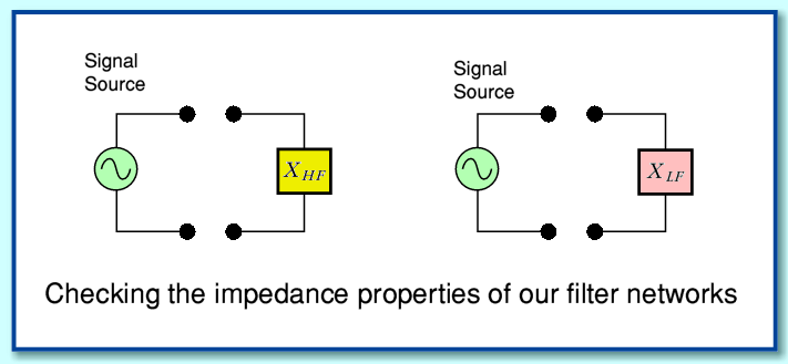
These networks have some interesting properties. If we look back to their defined impedance behaviour we find that they cannot have any power dissipation behaviour (i.e. resistance). The reason for this can be explained as follows.
Imagine the situations shown below where we take each of our filter networks and use a signal generator to check out their impedance properties. If we apply a test sinusoid with a frequency  then we find that
  behaves like it has an impedance of zero, and
  behaves like an impedance of infinity. This means that no matter what magnitude of current we apply, we can’t get any voltage difference between the terminals of
  . And no matter what magnitude of voltage we apply, we can’t get any current to flow through
  . This all follows from the ‘ideal’ properties we defined these filters to have earlier on.
Since the power dissipated in a resistance is equal to the the product of the voltage and the current we find that neither network actually dissipates any power. In one case because the current is zero, and in the other because the voltage is zero. If we now try a frequency  the roles of the filters swap over, but we get the same end result. Neither filter dissipates any power.
What the above tells us can be generalised since we can treat other waveforms as being composed as a series of sinusoidal frequency components. Every individual component will be unable to dissipate power in the filter networks. The impedances of both networks have no resistive component in which power can be dissipated.
Now lets consider what happens when we try a waveform which has a pair of frequency components, one above  and one below. In this situation one component will be able to produce a voltage between the filter’s terminals, and the other will be able to cause a current to flow through it. This means that the product of current and voltage won’t always be zero. However since the filter networks have no dissipation resistance what happens to this non-zero power level?
Let’s start with the monowired arrangement. The current though  is
is  , and the current through
  is
is  . The voltage across
  is
is
i.e. the amplifier output voltage minus the potential drops across the relevant resistances. Similarly, the voltage across  is
is
For the bi-wired arrangement we get the same current levels, but the voltages are slightly different as each cable now only sees the current for the relevant drive unit. Hence for the bi-wired case we get
i.e. the amplifier output voltage minus the potential drops across the relevant resistances. Similarly, the voltage across  is
is
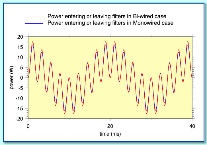
Using the expressions for our example of a signal with two sinusoidal components these become in the monowired arrangement:
and in the bi-wired arrangement:
As we might expect from the defined properties of the networks, no voltage component appears at the frequency for which a filter network has a series impedance of zero. We can now use the above to work out expressions for the relevant power levels. For monowiring
similarly, for bi-wiring
Using the same waveform with two frequency components as previously we can now plot the power levels for the filter networks in the two arrangements. This is illustrated above. Looking at the above plots we can notice two points. Firstly that these power levels can have either a positive or a negative value. Secondly, that their values for the monowired and bi-wired cases are similar, but not identical.
It is important to remember that – unlike the situation where we are considering resistances – the above power levels do not represent dissipation losses. This is because the filter networks, as a consequence of their defined properties, have no resistance so cannot dissipate any power. Hence when the above values are positive this represents the rate at which energy is stored within the filter network(s), and when they are negative it represents the rate at which energy stored within the filter network(s) is released back into the rest of the system. This behaviour is normal for ‘reactance’ and reactive elements (e.g. inductors and capacitors) generally exhibit this behaviour.
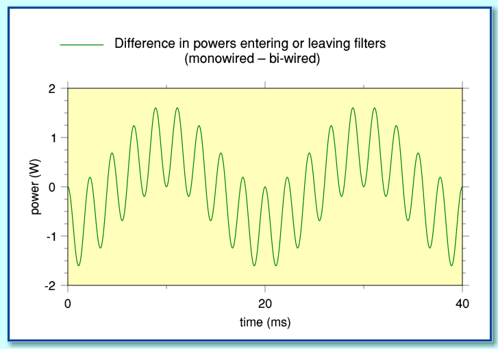
We can now define the difference
where the subscript ‘M’ indicates the monowired values and ‘B’ the bi-wired values. From this we obtain the result
For our chosen example signal the above illustrates this difference in filter network power levels between the monowired and bi-wired arrangements.
Now, if we now look back to the difference in cable dissipation levels between the monowired and bi-wired arrangements we discover that
What this tells us is as follows:
That although the monowired and bi-wired cases show patterns of cable energy dissipation levels which vary with time in different ways, this difference is equal and opposite to the difference in their patterns of energy storage and release in the reactances of the filter networks. In reality, the two arrangements differ in the details of temporary energy storage and release, and this alters the time variations in the power dissipation in the cables.
As a result, the two behaviours cancel out, and the two arrangements behave identically so far as the amplifier and speaker units are concerned. Thus if out interest is in comparing the arrangements for the task of conveying signals from the amplifier to the speaker units, then they are indistinguishable. The ‘internal’ details differ in terms of how energy is stored or dissipated, but this has no consequence so far as using the system is concerned.
The ‘conundrum’ outlined earlier – that the systems are the same so far as amplifier and speaker units are concerned, but the cable dissipation patterns differ – can now be seen in terms of the way the filter networks temporarily store and release energy as a consequence of their defined properties. No energy is mysteriously ‘lost’ or created out of nothing. All that is happening is that, as is usual with circuit elements with frequency dependent behaviour, some energy storage and release is involved.
Conclusions
Previous webpages have shown:
1) That monowired and bi-wired arrangements may produce different frequency (and phase) responses as a result of the changes in the impedance/network behaviours of the two arrangements.
2) That the presence of the ‘AB’ term in the cable power dissipation when we simultaneously have an HF and an LF current does not lead to any distortion or intermodulation of the kind stated in the web thread.
The above allows us to now add:
3) That the presence of the ‘AB’ term in the cable dissipation for the monowired arrangement does not mean that the systems produce different results.
It may seem strange that we find that – despite the ‘internal’ differences – the two arrangements behave identically so far as amplifier and speaker units are concerned. However this is a consequence of the properties of the chosen  filtering elements. i.e. that they should pass one band of frequencies with an impedance of zero, and block the other like an open circuit. This behaviour leads to the result of a system that is unaffected by the choice between monowired and bi-wired arrangements.
In practice it is not clear what filters we might build that would actually deliver the assumed ‘ideal’ behaviour. When we examine the behaviour with more practical filter networks we may therefore find the result does not show bi-wiring makes no difference so far as the amplifier or speaker units are concerned. Indeed, an example of a simple choice of filter elements has already been examined on other pages. In that case it was clear that changing from monowiring to bi-wiring arrangements may change the impedances in the system. This may then alter the frequency (and phase) response of the system. This result can be understood without having to take any interest in the apparent ‘anomaly’ in the power dissipation patterns in the cables. It is a consequence of any changes that arise in the current levels (or phases). However it is open to question if this is large enough an effect to be a real concern.
The claims made in the web thread focus on arguing that the difference in cable dissipations implies a difference in performance. The above shows that this isn’t the case. What may make a difference is that changes in impedances due to the non-ideal nature of the filter networks can alter the frequency response. This also shows up as a change in the levels (and/or phases) of the HF and LF currents. But you do not need to consider the cable losses or worry about an ‘AB’ term to show this. Indeed, such changes in response would show up with signals which consist of a sinewave where no ‘AB’ term could arise in the power dissipation.
The conundrum presented in the web thread is therefore essentially an irrelevance, based upon looking at the cable dissipations, and neglecting what happens at the actual amplifier, speaker units, and at the filter networks which are implicit in the situations being considered. The puzzle evaporates once the behaviour of the rest of the arrangements – in particular the filter networks – are taken into account. The conclusion is therefore that the claims made in the web thread do not provide any basis for arguing that monowiring and bi-wiring differ in their performance. The mystery is simply a product of focussing on an irrelevance without appropriately considering its context. If this were a detective story, we would end by discovering that nothing mysterious had actually happened!
Back to main Analog and Audio page.