How short is a piece of string?

When a connecting cable is very short we can estimate its effect upon signals by using a lumped model of its behaviour. For longer runs of cable this approach breaks down and we have to treat the cable as a transmission line. But how long is ‘short’?... This question is of particular interest for domestic audio systems where the cables are typically a few metres in length and the signal frequencies only extend to a few tens of kilohertz. In general, such systems are also used without matching - i.e. The source, load, and cable characteristic impedances are generally unequal - and the signal (information) pattern is represented by the voltage variations. The following analysis first works out the details of two models – lumped versus transmission line – and then compares the results they give for a situation similar to the use of loudspeaker cables in a domestic audio system.

The transmission line model

Figure 1 shows the basic model used to represent the behaviour of a single-mode linear transmission line. The values with a prime are assumed to be per unit length. The details of this model are discussed elsewhere. Here we can simply say that the CRLG values are equivalent to two complex values for the characteristic impedance,

, and propagation constant,

. The relationship is given by the expressions

Note that in general we can expect these values to be frequency dependent and complex.

In terms of conventional electronics circuit diagrams can represent a system where a source and load are linked by such a transmission line by the arrangement shown in Figure 2. However an alternative approach is useful if we wish to determine the effect of the transmission line on the (voltage) signal level which appears at the load. This is based on noting the similarity to various other physical systems like stacked optical media or loaded Fabry-Perot Resonators using reflectors with different reflectivity values.

Figure 3 illustrates the physical behaviour of such systems. Here we have two semi-reflecting boundaries spaced apart with a medium whose propagation properties are defined by the propagation constant,

. An input signal (generator voltage from the source),

, produces a series of signal contributions at the load. Each interface has a (voltage) reflection coefficient. From basic transmission line theory we can say that for the source-cable boundary the reflection and transmission coefficients for a signal incident from the source will be

Similarly, at the cable-load boundary, the equivalent values for a signal incident from the cable onto the source will be

From symmetry, the values for signals propagating in the other direction will experience reflection and transmission constant values of

Using these values, we can define the signal contributions reaching the load as shown in Figure 3. The total load voltage experienced will be

where

The above is a standard infinite series which is equivalent to

We can therefore define a voltage gain (actually a loss) ratio when the cable is used

Note, though, that this includes the effect of the source and load impedances which would still be present if the cable length were zero. If we wish to determine just the change in gain and hence signal level at the load caused by using the cable we can normalise with the factor

(The second expression is the gain when

equals zero – i.e. when the cable is of zero length, so has no loss or delay.) This allows us to obtain

which provides us with the change in signal level and phase at the load produced by the presence of the cable in the system. This result is an entirely analytical expression based upon the transmission line approach which does not depend upon approximating the cable as a series of elements.

The lumped model

The alternative approach is to pre-assume the cable is short enough to be regarded as a set of four lumped values as shown in Figure 4.

Where for a cable of length, d, we simply say that

i.e. choose CLRG by multiplying the values per unit length by the actual length. This is about the simplest lumped approximation we could employ to represent the cable. Better approximations would employ multiple elemental lumped stages and be arranged with symmetry. However I decided to use this simple model for the purpose of comparison with the analytical transmission line model.

Here the gain with the cable present will be

where

and the operator

represents parallel combination. i.e. such that

As before, the effect of the cable may be normalised against the behaviour due to the source and load when the cable is of zero length. Here this means that

where

Comparison of results

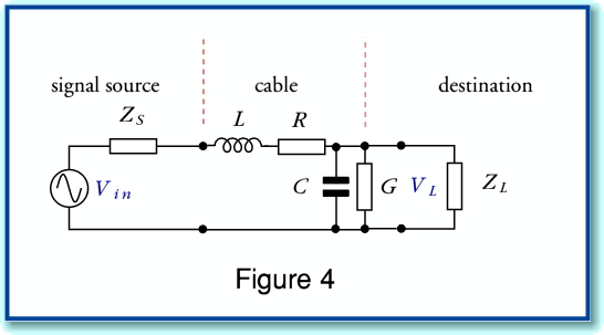
Having defined the two models - analytic transmission line versus simple lumped approximation – we can now compare the results they predict is a situation of a kind appropriate for domestic audio. For the sake of example we can consider a 5 metre run of various loudspeaker cables with an 8 Ohm load. For simplicity, the source impedance is assumed to be essentially zero. i.e. the power amplifier has a high damping factor and negligible output impedance.

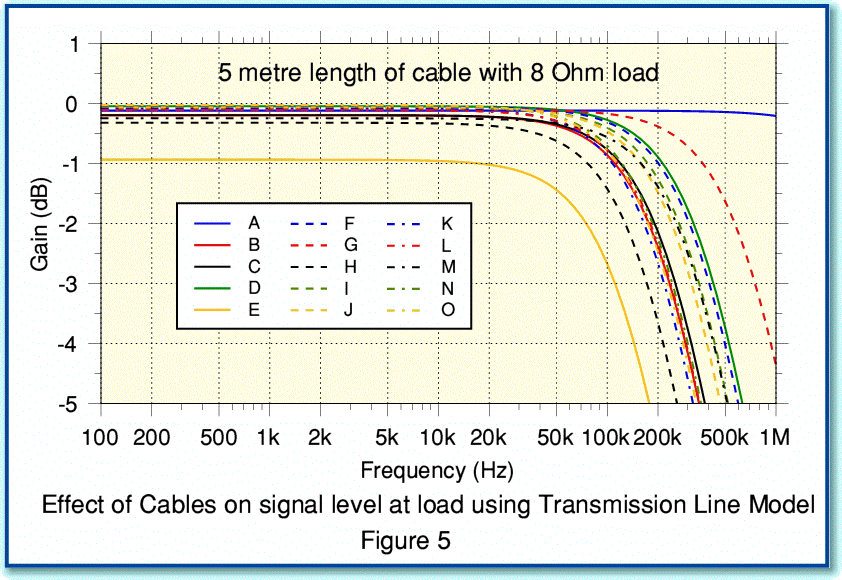
Figure 5 shows the change in signal level at the load predicted by using the analytical Transmission Line model. The results are for a random selection of 15 different loudspeaker cable designs whose RCGL values were measured and published in a survey in Hi Fi News some years ago. The measured values used in each case are listed in the table below.

Table of Cable Parameters

Cable	pF/m	microH/m	millOhms/m	1/MOhm/m
A	1500.00	0.11	22.00	500.00
B	34.60	1.06	36.20	250.00
C	41.60	0.98	36.40	140.00
D	170.00	0.60	8.40	55.00
E	44.80	1.99	182.00	250.00
F	88.00	0.63	10.60	67.50
G	143.40	0.34	18.20	500.00
H	20.00	1.42	60.00	150.00
I	48.00	0.72	14.00	300.00
J	48.00	0.80	11.40	85.00
K	59.20	1.16	15.20	61.00
L	58.00	1.06	20.00	55.00
M	36.00	0.72	46.00	500.00
N	28.00	1.04	7.60	250.00
O	26.40	1.11	4.60	165.00

You can see that changing the cable can alter the frequency response in the region above 20 kHz, and alters the overall level at lower frequencies.

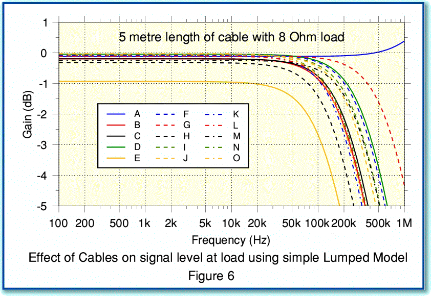
Figure 6 shows the changes in signal level for the same cable, but this time predicted using the simple Lumped Model. Comparing Figures 5 and 6 you can see some differences in predicted behaviour in the region above 20 kHz.

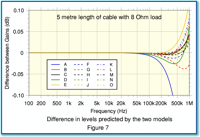
To make things clearer we can subtract one set of results from the other and display the differences. This will mean that 0dB will represent where the two methods give the same result, and any departure from 0dB indicates how much the two models disagree. The results are shown in Figure 7. Note the more sensitive vertical scale on this graph. From Figure 7 we can see that for our example conditions the two models produce much the same results for frequencies up to about 50 kHz. i.e. over a wider bandwidth that would be produced by most domestic audio sources. Even up to around 200 kHz the discrepancies between the two ways of predicting the effects of the cables give results similar to better than the 0.1 dB level.

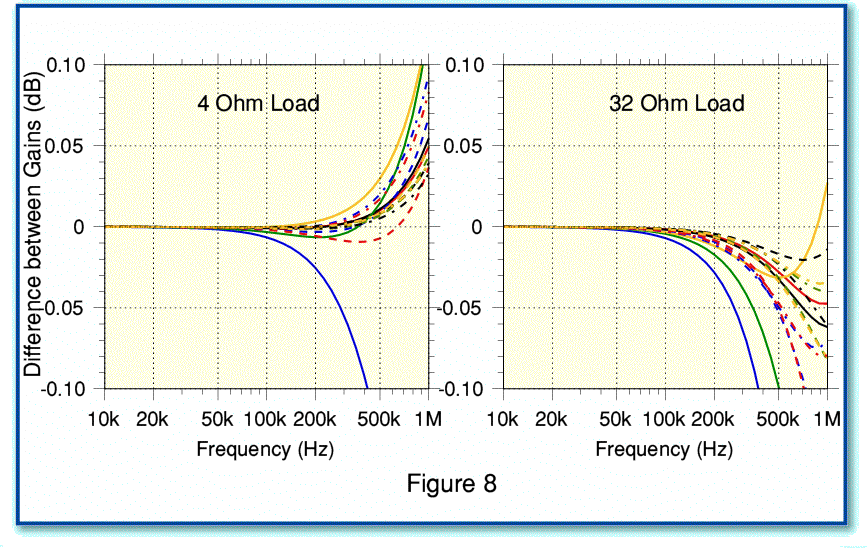
Figure 8 shows the difference in predicted levels for two alternative choices of test load using the same types and length of cable as previously. Although the details vary above 50 kHz you can see that these loads give the same basic behaviour as for 8 Ohms. i.e. that the two models give virtually identical predictions below about 50 kHz.

Of course, the above result might change if we used significantly longer cables, or loads whose impedance is nothing like 4 - 32 Ohms. But for cables somewhat shorter than 5 metres it seems likely that the simple lumped element approach will be fine for analysing the audio frequency behaviour of a cable. Hence in practice domestic loudspeaker cables a few metres long can be regarded as being short enough to for us not to need a transmission line analysis to model their effects upon signals at audible frequencies.

Jim Lesurf
28th Aug 2008

Click here to go to the Analogue and Audio Homepage