Outline of method used for numerical/computer
modelling of hearing sensors.
An explanation of how the results shown on the main ‘ringing in the ears’ pages were obtained can be given in two parts. The first is conceptual and outlines the physical assumptions in terms of the analog electronic analogy for a simple bandpass resonator. The second part outlines the program method which employs an equivalent technique. In each case, the approach is based upon a number of similar analyses of non-linear and linear systems I’ve examined in the past in other areas. Hence the methods are fairly standard, but some may be fresh applications to this specific topic. The explanations given here are just a brief outline and omit details and background for the sake of brevity.
Conceptual
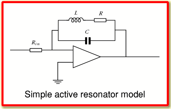
The basic standard anology for an active resonant bandpass system is as illustrated below.
The gain and bandwidth of the above system depend upon the value of the resonator loss resistance,  , compared with the impedance of the inductance,
  , at the resonant frequency The resonant peak frequency is determined by the
  and
and  values. The lower the value of
  , the higher will be the
  of the resonance – i.e. higher gain and narrower bandwidth. In terms of general physics, resistance in the RCL loop acts as an energy dissipation mechanism. The capacitance and inductance act as energy storage mechanisms. The lower the amount of loss (resistance) compared with the amount of capacitance and inductance, then the more energy the system can store. In dynamic terms, with such a system the stored energy level grows until the rate of loss due to the resistance matches the rate of loss due to resistance. Thus a low value for the resistance, R, implies a high stored level (and hence gain), a longer response time, and a narrower bandwidth of response.
In most electronic filters the output voltage would then be passed to something like a square-law device or other power detector to obtain a value which, when time averaged appropriately, would indicate the detected power integrated up to the time. However a better measure in general for physical systems is to monitor the stored energy in the resonator which is given by an expression of the form
where  is the current through the inductor and
  is the potential difference across the capacitor. This measure has the advantage that it does not vary from a maximum to zero twice during every cycle as the stored energy is transferred back and forth between the magnetic field around the inductor and the electric field between the plates of the capacitor. In general physics terms, resonators are systems where energy is regularly transferred back and forth between two storage mechanisms and may some may be dissipated in the process. Familiar electronic circuits are just one example of this general physical process. Hence, for example, the analogy between an electronic resonator and something like a gravity pendulum.
For a linear model we would assume that all the circuit values are constant, and are unaffected by the signal levels. Hence such a circuit with constant values may be used when we wish to model the behaviour of human hearing with the assumption that the system acts in a linear manner.
To represent a nonlinear model of human hearing is it is useful to make two changes to the conceptual circuit.
- Firstly, we balance the energy dissipations so that loss occurs at the same rate from each energy storage mechanism. This means we now have two resonator dissipation loads with values chosen appropriately. In terms of an electronic circuit this would mean adding another resistance, placed in parallel with the capacitance, and choosing its value appropriately.
- Secondly, we now arrange for these dissipation resistance values to change in response to variations in the stored energy levels. This introduces the required nonlinearity. For the hearing model, we arrange for the loss (i.e. the
 ) to incease with the stored energy level, and then regard the stored energy level as the measure of the detected response of the resulting nonlinear system.
Numerical model
The method employed for computation of the results was based upon a time-step update approach, This essentially replaces the relevant nonlinear differential equations that would describe the the system with a set of equivalent equations specifying the changes that occur in small, but finite, time step intervals.
Rather that do a time-step model directly of the above it is simpler to treat the system as being frequency converted down to two ‘d.c.’ values. This is analagous to using a biphase PSD to sense the two energy storage levels. An example of this usage is when this form of conversion is used during signal processing to synthesise filters. It allows us to mimic a bandpass filter in terms of down conversion followed by a low pass filter.
Here the sensor state is represented by two values  and
and  which are initially set to zero and then each time a new data value arrives we update using the following steps.
1) take each new input value,  , at time
  and perform
where  is the time step in between successive samples and
  is the centre frequency of our resonant bandpass filter.
2) Now rescale the two values by a value slightly smaller than unity to introduce the dissipation losses that give the system a finite gain and bandwidth. i.e.
The loss factor here is determined by
where  is a factor determined by the most recently sensed signal level and
  .
.
The above means that by varying  we are altering both the effective gain and the effective bandwidth since the smaller the loss, the longer the integration time of the resonator storage.
3) update
where  is a chosen power for our nonlinearity.
 would suppress any nonlinearity. Values of
  in the range 1·5 to 3 may be justfied by various aspects of the hearing models in the literature, etc. However tests seem to show the chosen power-law value does not matter a great deal once you are above unity and chose ‘reasonable’ values implied by the literature.
Now loop forwards for the next input  and
and  values. Also if required add a time smoothing to the time variations of
  .
.