In a Dither

Despite Audio CD (CD-A) having been with us for over twenty years it remains routine to read misrepresentations of how it works and incorrect claims about technical ‘problems’ with digital audio. Having become a bit weary of repeatedly seeing statements in audio magazines that can be shown to be wrong both by formal information theory, and by measurements, I decided it might be useful to try and give a clearer explanation of some of these points.

In my experience the most common pair of errors people make in magazines when describing CD-A are of two types:

The digital samples must lose tiny details as a result of ‘truncation’ or ‘quantisation’. This is sometimes contrasted with ‘analog’ systems which are (mistakenly) assumed to have ‘infinite resolution’.
Below about -60dB music on CD-A becomes distorted.

Graphs and measurements in audio magazines are also sometimes presented which are either not clearly explained, or used to give misleading values and incorrect conclusions.

It is possible using the formal mathematical methods of Information Theory to show that both the above statements are at best misleading, and provided sampling is done correctly, simply false. By reference to the work of Shannon and others, the assumptions about both ‘digital samples’ and ‘analog’ behind the above statements can also be seen to be false. However rather than applying a formal mathematical approach I’d like to illustrate these points by using some examples. To do so, I’ll start with a brief description of the digital sampling process as used for CD-A.

CD-A and sampling

CD-A sets out to provide recorded sound in a stereo format. Thus there are two ‘channels’ – left and right. Here I’ll ignore that and just consider one channel. The descriptions I give below are them duplicated for a second channel when we want ‘stereo’.

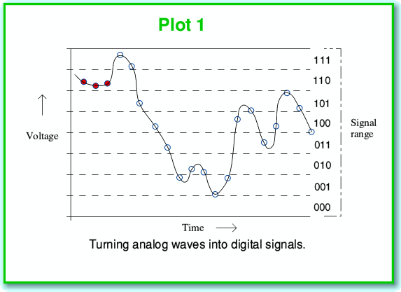
We can represent the sound information in terms of a required time-varying pattern or ‘waveform’ of how the air pressure changes with time. In ‘analog’ systems we use a continually varying voltage or some other property and arrange for this to vary with time in the same pattern as the required sound pressure variations. In ‘digital’ systems we make repeated measurements of this pressure (or voltage) at a series of equally spaced instants, and note down the values we obtain. This series of values then represents the pattern. This process is represented in the above diagram (Plot 1) where each sampled instant and value is represented by a small circle on the continuous wavy line that represents the actual pressure or voltage variations with time. The process considers a given range of possible pressure levels and divides this range up into a series of narrow ‘bands’. It then assigns a number to each band as a sort of label. In the example shown above we can then write down the series of number labels – in this case as 110, 110, 110, 111, 111, etc...

Here I’ve just used 3-digit binary values for my numbers or labels. CD-A uses 16-bit binary numbers, so we can have 2¹⁶= 65536 bands. This means if, for example, we want to represent voltages in the range from +2·0 to -2·0 volts we wound find that each band is just over 61 microvolts high. This is quite a fine resolution and would show up small changes, but it is limited, and this leads to the problem which we again see in the above illustration. For the sake of example I’ve coloured the first three sampled instants with red-filled circles. If we look at these we can see that although the signal does wiggle about a little during this short period of time, the variations leave the first three sampled instants in the same band. Hence the first three values in our sequence are the same, and show no signs of the fine details of the waveform variations during the period when this first three sampled were taken. Information was lost. This process where each individual sample value covers a small but finite range of possible pressures or voltages is called ‘quantisation’. Any loss of details or errors due to this are then said to be due to this process.

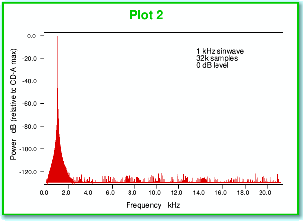
We can see this potential problem in another way by looking at the power-frequency spectrum shown in Plot 2, below. Note that here, and for the following examples, I have assumed we have taken waveforms and sampled them in the manner used for CD-A – i.e. at a sampling rate of 44,100 samples/second, and then represented the results as a series of16-bit binary integers. (In fact since we have to use one bit to indicate if the sample value is positive or negative we only have 15 bits for the rest of each number.) The plots of spectra are taken from a series of 32,768 successive 16-bit samples, so corresponds to a series of values lasting just 743 milliseconds. This particular number of samples has been chosen for all the results shown on these pages as this is convenient for the process (Fast Fourier Transformation) that is used to work out the spectra. It is also typical of the kinds of results presented in audio magazines.

The signal used for the above power-frequency spectrum was chosen to be a sinewave with the largest amplitude we could record without clipping. It therefore swings up and down over all the 65536 levels which CD-A can record. If the recording process were ‘perfect’ we’d expect to only see one item on the spectrum. This would be a spike at the 1 kHz frequency, and nothing else. In reality, though, we get a lot of ‘grass’ along the bottom of the spectrum, showing some power at all sorts of frequencies reaching up to over 20 kHz. These have appeared because of the quantisation we described earlier. In effect, these unintended components in the spectrum represent distortion. We’ve allowed the quantisation to create extra frequencies that were not in our original waveform.

With large signal variations like the 0 dB sinewave these distortions are at relatively low levels. Looking at the above plot we can see that they all sit well below the -120dB level. This means that each distortion component is a million million times weaker than the main signal. Hence in this specific situation we might feel the problem isn’t worth worrying about. Alas, music and other sounds tend to vary in loudness. When we have to deal with quieter sounds we find that - unless dealt with – the problem can become rather more serious.

Given the above it is quite understandable why some of the people who write in audio magazines seem to regard this as a fundamental problem. However in fact it is not. for reasons which I hope should become clear from the explanations and examples I can give below. The ‘magic’ which some audio writers fail to take into account stems from two points;

That all real quantities we measure come with some superimposed ‘noise’ – uncontrolled and random (unpredictable) fluctuations that fog our ability to make any measurements of varying quantities with high precision. Hence our ability to resolve arbitrarily small details of a real analog signal pattern is limited, and we can’t expect infinite resolution.
The techniques known as ’dither’ and ’noise shaping’. These exploit noise-like patterns to deal with the above truncation or quantisation problem.

Page 1 of 4