Challenge and Response
In this part of my investigation I want to look into the question of what changes MQA may make to ‘High Resolution’ (HR) audio material as a result of it being run though an MQA encoder and decoder. The definition of HR in this context means either employing a higher sample rate than 44·1k or 48k and/or more 16 bits per LPCM sample (typically 24 bits). Here the emphasis will tend to be on the use of a higher sample rate as, in practice that tends to be what attracts listeners due to the implicit promise of a wider frequency range – and hence also improved temporal resolution.
The main difficulty here is the same as affected my previous investigation[1] – i.e. the challenge of finding examples of what we can be confident is exactly what was put into the encoder. (If you haven’t already done so, I’d suggest reading that page first as it may help set the context of what follows here.) However we do currently have one example which is worth examining because it has been said to provide precisely the required input and output examples. This is a set of files made available by ‘Golden One’ (GO) and has been the topic of discussions on at least two web forums - Audio Science Review[2] and Pink Fish Media[3] in threads discussing MQA. That said, the only ‘provenance’ we have for this is the statements of GO which I have no independent means to check. So for the purpose of this investigation I will take the files ‘as supplied and described’ and see what the results may show.
Golden One
If I understand correctly, GO initially created an ‘Original Master’ file in 88·2k/24bit LPCM format. From this he then created a downsampled ‘Original Master’ of the material in 44·1k/24bit LPCM format. The content of the downsampled version nominally being identical to that of the 88·2k version except for the loss of any information components above the Nyquist frequency of 44·1k sampling. i.e. everything above 22.05 kHz would be lost.
He then submitted both files to Tidal for encoding and streaming, then fetched copies of the results from Tidal in two nominal forms – MQA and ‘Tidal’ (non MQA). He then used an MQA decoder to render output for comparison with the source files he submitted. Here for the purpose of investigation I will assume this is what occurred.
The table below summarises the main details of these files.
| File | rate | bps | Duration | Size | Impulse at |
| Original Masters 44k range content | 88·2 | 24 | 300·8851 | 152M | 7,417,658 (1:24·10043) |
| MQA encoded 44k range content | 44·1 | 24 | 300.8851 | 76M | 3,708,831 (1:24·1005) |
| Tidal version 44k range content | 44·1 | 16 | 300.8851 | 51M | 3,708,831 (1:24·1005) |
| Unfolded 44k range content | 88·2 | 24 | 303.1500 | 153M | 7,564,660 (1:25·76722)* |
| Original Masters 22k range content | 44·1 | 24 | 480·4731 | 121M | 2,910,207 (1:05·99111) |
| MQA Encoded 22k range content | 44·1 | 16 | 480·4731 | 81M | starts 2,910,207 (1:05·9911) peaks 2,910,212 ends after 2,910,305 (approx 1:06) |
| Tidal version 22k range content | 44·1 | 16 | 480·4731 | 81M | as above |
| Unfolded 22k range content (nominally) |
88·2 | 24 | 375·1648 | 189M | starts 2,975,332 (1:07·4678) lasts about 100 samples |
* = Track starts with a series of zero samples. First non-zero sample # 153,797 (1·7437)
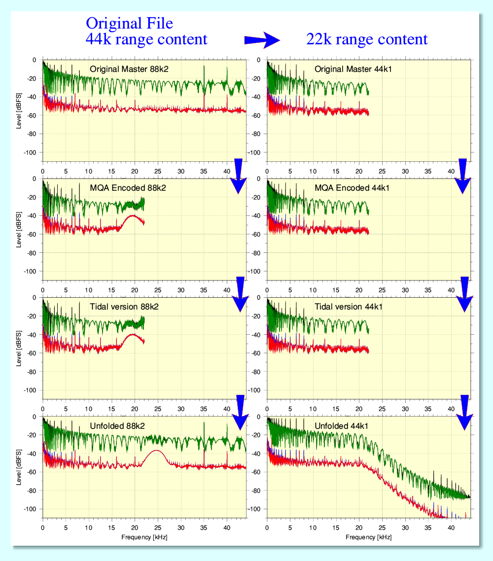
The above show average and peak FFT spectra of the various files. The blue arrows indicate what I understand to be the ‘family tree’ of how they are related. On each graph the time-averaged levels for the Left and Right channels are plotted in red and blue. The peak levels found for any individual FFT are plotted in green and black. Note that for these graphs the channels essentially overlay so you only see one channel’s plots as they cover the results for the other.
These spectra were calculated in a similar way to the example shown on the previous page that dealt with 2L examples. Note, however, that they all use the same number of samples per FFT. This means that width of the frequency ‘bins’ depends on the sample rate of the source file, and that this also means that the levels may be lower as a result for the 44·1k rate files - i.e. the ones that only extend half-way across their plot. This, and the lack of precise time-alignment should be kept in mind when comparing the various examples shown above.
We can see that these files aren’t all identical in duration. And the presence of an isolated impulse function in them also shows a lack of time alignment. I don’t know why this occurs, but it does complicate analysis, as did similar differences amongst the 2L examples I have already analysed. The spectra also show a number of differences between the various files. One curio is that one Original Master file was a 44·1k rate file. Yet despite having no HF above it’s Nyquist limit (22kHz) it was apparently decoded by MQA. The result created an HF content which was absent in the source file. I have no idea why this occurred, but if the file was streamed by Tidal as ‘MQA’ this is presumably the result of it being given an MQA ‘key pattern’ that told the MQA decoder to duly ‘unfold’ this HF. If so the process seems surprisingly mechanistic in its response.
An obvious difference between the files is in that the ones stemming from the 88·2k Original Master we can see a process noise ‘bump’ becomes added in the region around about 24kHz. This is similar to a lower level equivalent that is noticeable in some of the 2L files. It presumably is a result of the method used to ‘hide’ HF info by the MQA system and remains present in the end-result.
Files with 22k-range content.
Here I will look at the files that include no original content above 22kHz. (i.e. The ones on the right in the above diagram.) This is convenient because their MQA encoded and unfolded examples lack the high levels of added process noise which makes analysis of the full-44k-range content examples difficult.
The files include an isolated impulse function which can be used to probe the impulse response – and hence any linear process filters – in a signal chain.
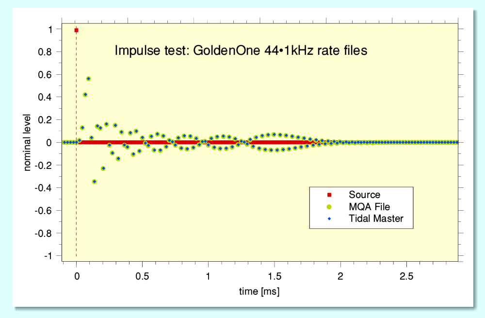
The above summarises the results for the source file which was sent to Tidal as a plain 44·1k file that has no content whatsoever above 22·05kHz. (In the plots shown below Left and Right channels are both plotted, but are actually indentical, so in each case only one channel is visible.)
The input (red square blobs) is a single non-zero sample impulse. The time-aligned results for three files are plotted on the above graph. The input is said by GoldenOne to be from what was sent to tidal. The other two are for the ’Tidal Masters’ and the ’MQA’ versions which resulted from the 44·1k sent in. These both show a considerably amount of dispersion, and are essentially identical! This result is very strange for two reasons:
The impression given is that this means that – although labelled differently – both ‘output’ versions obtained from Tidal are actually the same and both have dispersion added which was absent from the source material. To check this I did a sample-by-sample subtraction of the contents of the files and got a series of zeros. This confirmed that, regardless of their Tidal labels, the two files are identical. In effect, the version not identified as MQA would seem to be MQA encoded.
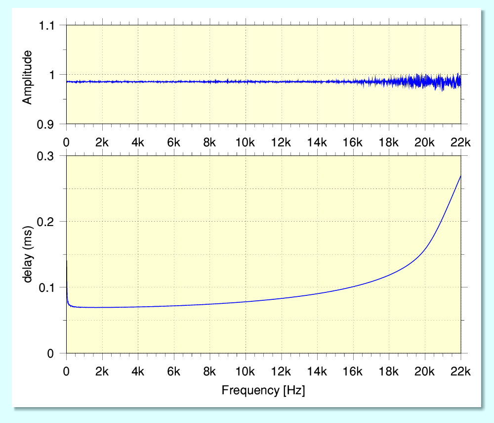
Having found the impulse response function in the MQA encoded file(s) which the input impulse had swept out I used this data to calculate the frequency-domain response of the filter that had been applied. This gave the above results. You can see that the amplitude response is close to being flat. (N.B. The input impulse is slightly below 0dBFS. If this is taken into account the amplitude gain of this filter seems to be essentially unity.) But the filter produces a dispersion of around 0·2 msec across the range from near-dc to 22kHz. What isn’t clear is: Was this dispersion been added by Tidal for some reason? If so, why? If not, was it added by the MQA encoding, and if so, why? Either way it seems strange given the concern MQA express about ‘de-blurring’ – quite the opposite of which is exhibited in this example. That said, because of the distribution of the impulse response pattern the group delay spread is lower than might be the case. But the puzzle is why it happens at all!
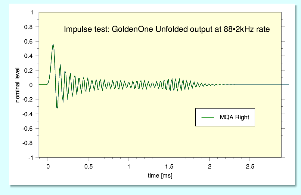
I then performed a similar process using the impulse response in the ‘unfolded’ result produced by MQA decoding. The overall resulting impulse response was as shown above. This is also clearly dispersive and time asymmetric.
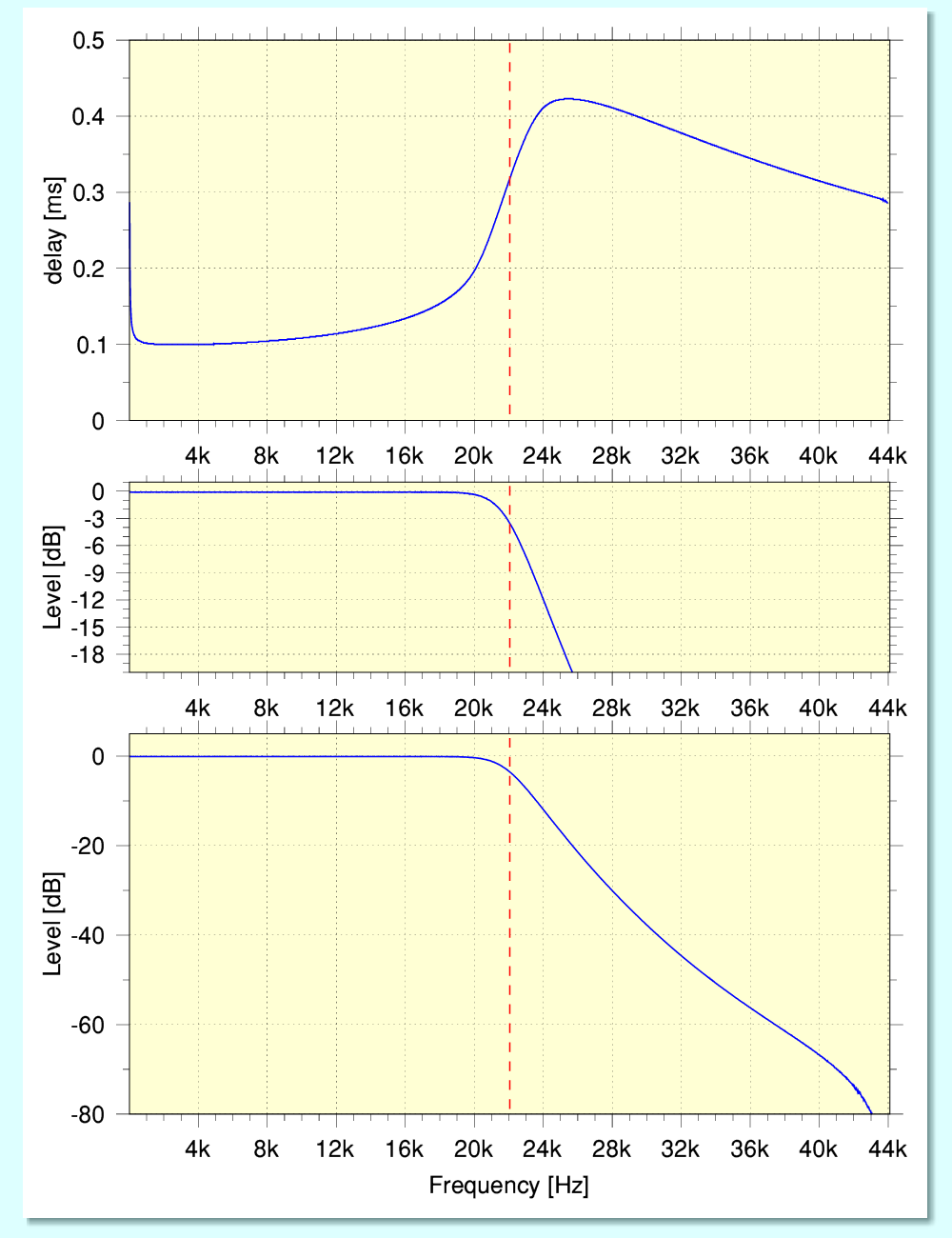
The above shows the results of deriving the related filter behaviour represented by the impulse response. The surprise here is twofold
I have added a broken red line to the above graphs at 22·05kHz to make this point clearer. In essence, output to the right of this line was added by the MQA encoding-decoding process. This might perhaps ‘spice up’ the sound but simply wasn’t in the ‘Master’ which preceded it!
Note this response is nominally the convolution (combination) of the filtering applied by the encoder and decoder. In principle, given both these shapes we can deconvolve the two filters. But is it their combination that affects the output. In this example the result does not seem to correct or undo the dispersion which the encoding filter applied. I had initially thought that it would do so, but apparently not. The result seems to be that what gets played has a dispersion of between 0·2 and 0·3 milliseconds applied to it compared with the input. Again this was real a surprise given that MQA make a point of the importance they place on ‘de-blurring’ (their term) the ADC used to make recordings to get what they regard as optimum timing. I can only speculate that perhaps the dispersion is intended to avoid the ‘peaking’ of a transient leading to clipping. Yet if the above is normal for MQA any benefit of ‘de-blurring’ would be degraded by the added dispersion shown above. That said, I’ve been told that MQA actually employs a range of selectable filters, so maybe other filters don’t add the dispersion which seems to be imposed here. However even if so, it still seems odd that any of their filters should do this.
It is of course, possible that the above finding is incorrect for some reason, or that something about the file ‘upset’ the encoder. But this second possibility does seem strange given that the Original Master input in this case was actually completely lacking in any content above 22 kHz. So there as actually no HF to encode or overload the encoder. If the absence was a problem I’d have assumed/hoped the encoder would detect it and then default to simply passing though the input without any alterations. Perhaps flagging this in the process to alert someone. That would then have ‘failed safe’ rather than create the additions and alterations shown above. I would have said that a file at 88k2 rate that contained no HF above 22·05kHz should have been easy to detect and simply leave untouched. Albeit that it might then not be able to be sold labelled as ‘MQA’.
The above looks at the results obtained from a source file that had no content above 22·05 kHz. I began with that because those files were easier to analyse. The companion files which do contain genuine HF components generated encoded output that is far harder to examine, but some hints and information from the above does help set the context when considering the files that do carry HF, and provide some hints as to what may be happening.
The 44k-content files
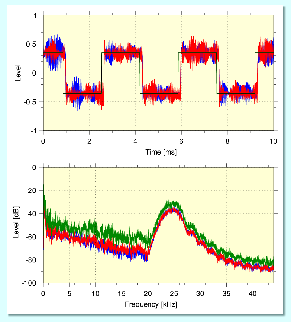
The 88·2kHz sample rate original source file and its resulting MQA encoded-decoded result are very difficult to assess because the result is quite dramatic! The above indicates why. The plots were obtained from a section of the file which contains a low-frequency squarewave.
The upper plot shows the waveforms (not quite time-aligned). The black line shows the waveform in the Original 88·2kHz master. The red and blue lines show the waveforms in the MQA decoded result. The high level of added noise is quite obvious. The lower graph shows the resulting spectra in the MQA decoded result. The added process noise is largely at high frequencies but it tends to swamp being able to examine the squarewave.
As an experiment I employed the ‘sox’ utility program to generate 44k-rate versions of both files. This removes most of the ‘hill’ – on in this case more like a ‘mountain’ of HF process noise from the MQA unfolded version and makes a comparison analysis easier, albeit one that focuses only on what can he provided by plain 44k LPCM. Note that any processing signature of the sox conversion should be common-mode for the examples compared here so should not affect the results that follow.
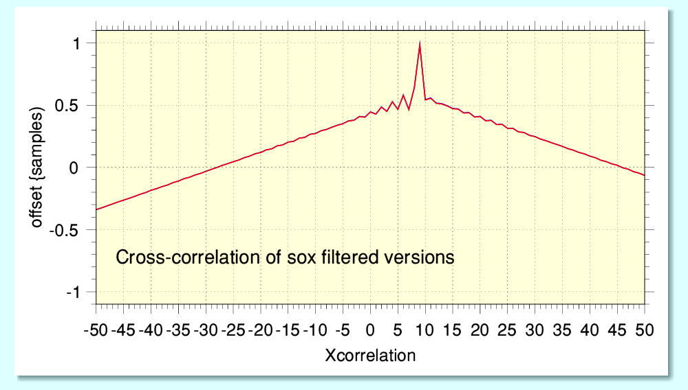
By a combination of inspection of the contents and some preliminary cross-correlations I obtained the above result. In this case I was able to pre-align the two versions well enough for their alignment to occur at about 9 samples away from the nominal data alignment of the correlation. This was good enough for the results to be clear.
I chose a 30 second section of the two files (which are, as provided, not time-aligned, nor of the same duration) which began with a burst of wideband noise. This is because noise tends to give a clear correlation peak if it is much the same in the two versions being compared. The narrow peak in the above result is therefore what we would expect to see if this is the case. i.e. it indicates that the part of the original noise below about 22kHz survives the MQA encoding-decoding process quite well. The peak sits on a triangular hill, which is what we can expect to arise as a result of a nominal squarewave elsewhere in the correlated sections.
The peak shows two useful features. The most obvious is that it reaches to almost exactly unity, which would represent a perfect correlation identity. (The correlation peak value is just over 0·98.) So we can say that if we are only concerned about below about 20kHz and regard anything above that as inaudible, then the decoded MQA is virtually a copy of the original master. This situation is similar to the 2L examples I have considered previously. In terms of just accessing the standard bandwidth audio the MQA process is ‘Mostly harmless’ if we reject > 20kHz – even in this extreme case which is a bit of a car crash so far as the response as HF is concerned, generating a huge amount of HF process noise in the high resolution output! The snag, of course, is that in this case it is also “mostly useless” in terms of getting the original input HF above 20kHz.
Less obvious is that the central peak is asymmetric and you can see distinct ‘ripples’ more prominently on one shoulder than on the other. This is a classic sign of dispersion. It indicates that MQA (or Tidal) applied a dispersive filter which affects the output decoded by MQA. Which is very strange given that MQA make a point of being both able, and keen to ‘de-blur’ ADCs, etc. Yet it seems that MQA itself ‘blurs’ the results it outputs in these examples. This may also help explain some of the features of the 2L comparisons I made and reported on my previous page on MQA.
Personally, I doubt I can hear the components above 22kHz in either case. However they may still matter because their presence may have effects which are not a part of the MQA process in itself...
Coda
I’d originally assumed that the effect of the MQA encoding-decoding process upon GO’s true-88k file meant that the full resulting output was too ‘damaged’ to be worth examining in detail. This assumption stemmed from MQA/Tidal’s comments to the effect that it over-stressed MQA and thus produced damaged output, and prompted me to try sox-filtered (i.e. downsampled) versions which lose most of the excessive added process noise. However upon seeing and reflecting upon the results I obtained from sox-filtered versions I re-considered this view.
The filtered versions cross-correlated quite well and gave a peak value close to unity. And the ‘damage’ which seemed to swamp the output ‘unfolded’ version was not only mainly at high frequency. It is also, of course, totally absent in the original source file. One of the properties of cross-correlation is that it tends to ‘see though’ any patterns which are absent in one of the versions being compared. Given this I realised that the filtered results implied that it was, indeed, worth doing a cross correlation of the 88k Input GO Master and the ‘unfolded’ version that emerged from running that though MQA encoding and decoding.
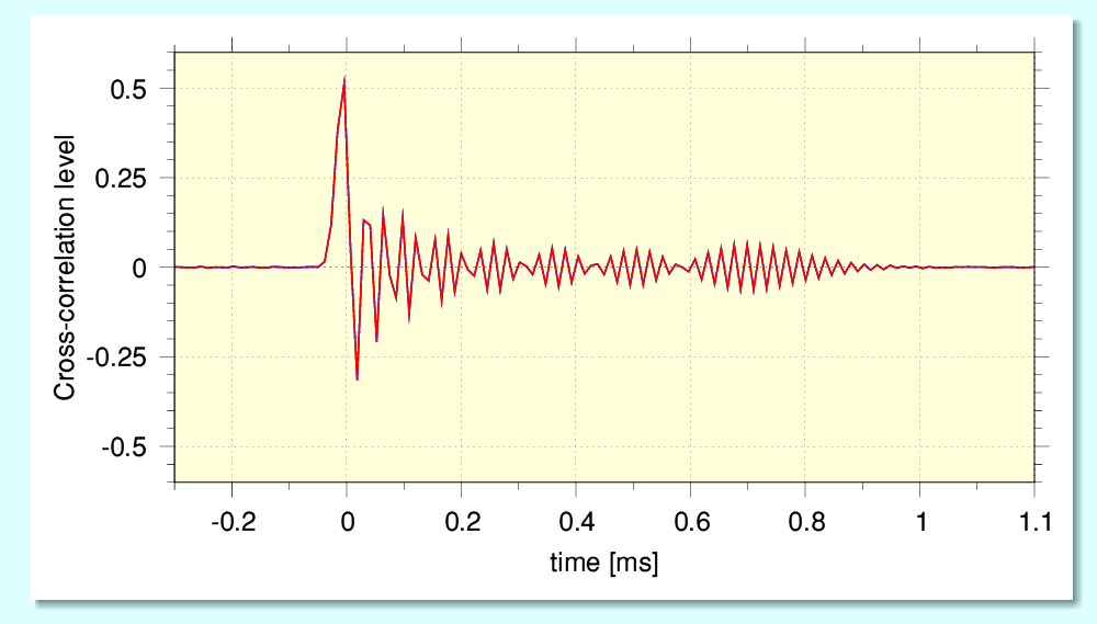
I chose the sections of the files which contain a burst of noise because a wideband noise signal is good basis for cross-correlation analysis. The above shows the result. It clearly shows a now-familiar pattern. This indicates that, yet again, the output version has had a dispersion filter applied whose effect is not removed or corrected by MQA decoding! Fortunately the MQA process does a fair job of making the added process noise ‘randomised’ so far as cross-correlation is concerned. Thus this pattern can emerge clearly despite the excessively high levels of process noise.
The persistent behaviour of having MQA add dispersion does raise a question: When someone compares an MQA file with a non-MQA high rate version of the same nominal content, might they hear a difference that is actually due to the dispersion? i.e. NOT due to the ways in which MQA tried to bundle HF into a smaller file, but simply due to the effects of the dispersion? This may then cloud over attempts to decide what the impact on the audible results may be of the file size compression-expansion methods employed by MQA. And – as elsewhere – this apparently blanket application of dispersion remains odd given the stated wish to ‘de-blur’ whilst apparently automatically adding dispersion. It seems to contradict the axioms of Information Theory!
The spectra I have plotted of the contents of the various files show the content divided into 4096 frequency ‘bins’. This helps make clear the overall spectral distribution of the content. However from an audio point-of-view we can make a more basic distinction between the traditionally ‘audible’ and ‘ultrasonic’ ranges of frequency. For the sake of a simple example I’ll assume ‘audible’ to mean up to 22kHz because this is the traditional sort of range over which Hi-Fi equipment has traditionally tended to be checked in terms of measurements, and is the nominal bandwidth for RedBook Audio CD.
If we revisit the example of a spectrum from the GO MQA-unfolded file that resulted from encoding the source file with content up to 44kHz we can calculate the total averaged power levels in the ranges above and below 22 kHz. That gives the following results:
| Frequency range | Left total | Right total |
| 0 - 22kHz | -18·0dB | -17·9dB |
| > 22kHz | -12·9dB | -12·8dB |
This shows that the overall average levels of ‘ultrasonic’ output is about four times bigger than that in the ‘audible’ range! More generally, on average music tends to have far lower levels of power above 22kHz than below it – which is a statistical fact MQA sets out to exploit albeit despite the risk that some music may not fit neatly into this class. Indeed, their approach implicitly requires this to be the case. (Hence their objection to GO’s test files.)
Now to be clear: yes, this is an extreme, exceptional case so certainly can’t be taken as representing what will typically happen in normal use! However it does raise a question about the possibility that in some ‘music’ cases the ‘ultrasonic’ power levels may be increased by MQA and then be high enough to justify considering the possible effect that has upon following items like, for example, loudspeaker tweeters or ‘digital’ power amplifiers. For example, it is common for loudspeaker ‘tweeters’ to exhibit large break-up resonance effects at frequencies above 20kHz.
At the time that I write this the current issue of Hi-Fi News magazine has reviews on various loudspeaker designs. The spectra of their output shows responses up to 60kHz. And in each case the region between 20kHz and 60kHz shows a resonant peak. In one case a peak that goes more than 20dB above the level at lower frequencies! And this is a costly, highly regarded, speaker design.
If nothing else, this indicates that the level of HF sound output in this resonance range will be emphasised. So if the listeners can hear audio at these frequencies this resonant peak may affect their enjoyment. (And, of course, if they can’t hear this then the presence of the unfolded wideband audio isn’t something they actually need.) However it also tends to be the case that such resonances may be nonlinear in their behaviour. As a result driving the resonance can generate various forms of distortion that may then produce audible components at lower frequencies. As per the old saying: “The wider you open the window, the more muck flies in!”
In addition to this, the reality is that the power-handling capability of tweeters tends to be much lower than that of the speaker units which handle the lower frequencies. In effect, it take a much lower sustained power level to fry or alter the behaviour of a tweeter than a woofer. In general for music this doesn’t matter because speakers are designed to cope with music and speech. But the MQA encoding-decoding process may add some process noise at HF which existing speakers haven’t been consciously designed to cope with. So the level of process noise which emerges from MQA decoding at the relevant frequencies is something that needs careful consideration. The challenge being to determine what levels are typical and also what is the ‘worst case’ that someone with a large selection of material may face. As it stands when I write this, we don’t have any formal model which speaker designers or reviewers may use for this. They may have to learn by – potentially unfortunate – experience. So given an apparent lack of test results on this thus far it is something I may look into soon...
It has been reported that the MQA encoder reacted to GO’s 88k-content input file’s content by locating its control/indicator stream at the 12th-bit level. If I understand correctly this is usually located down in the 16th-bit level. The consequence is an exceptionally high overall process noise level. But the result seems to share with some 2L examples a resulting noise ‘bump’ in the 20 - 30 kHz region when ‘unfolded’.
Golden One’s files were removed from being available from Tidal. Again I have been told that they, and MQA, feel the files submitted by Golden One are essentially ‘not music’ and thus the MQA encoder can’t be expected to encode them and provide satisfactory results in audio terms.
My own view on that point is less absolutist. It seems a fair comment that it was, indeed, a test file aimed at finding the limits of the system and seeing how MQA performed, it was not intended as something to be enjoyed as music. On that level I agree with what I understand MQA/Tidal may have said. However against the files it do enable us to assess the fact that the system does have its limits, and to see how it operates when ‘stressed’ which I think is a legitimate purpose. This, to me, seems just as reasonable as the kinds of tests I would, for example, have routinely employed when testing power amplifier designs, There I’d try everything from playing high power square waves into a ‘difficult’ load, to putting the amp into a freezer overnight and seeing if that upset the performance, to repeatedly applying a screwdriver to its output terminals when it was playing to establish that it would survive a short with no damage. Yes, some tests may cause damage or snags/limits to manifest. That’s the purpose of some tests - to determine the limits of what a system can handle, and to see if it fails gracefully or not. Better to know your amp will blow a fuse than to find it sets fire to the buyer’s home. All this despite it’s use being to play music in someone’s home.
From a posting GO made later on the Audio Science Review forum I understand that he subsequently submitted a file that just contained a 1kHz sinewave at -3dBFS level. This was apparently rejected and Tidal refused to provide an encoded version. If this is the case it does seem needlessly defensive on Tidal (or MQA’s ?) part. I can’t see that it would have ‘stressed’ the MQA system. If they had a good technical reason I have no idea what it may have been as I write this.
In addition I would add the following points.
It would seem that Tidal happily encoded the original files and made them available. However if the content was ‘unencodable’ because it wasn’t ‘music’ I’d have hoped/expected two things to have happened at the time of encoding. The encoders should have issued a warning or alert, and this should have caused Tidal not to release the result without comment at the time. Clearly at least one of these expectations were not fulfilled. This is worrying if – as has been said – a large media company has already swiftly MQA encoded a large number of audio files. It raises a possibility that some of them may, also, ‘not be music’ so far as their encoder was concerned and as yet this hasn’t been detected or redressed. More generally, the idea that an encoder can decide what is, or is not, ‘music’ seems to me to be a non-trivial issue. And given the assumptions/claims made for the sake of MQA this is a question I hope to address at some future point. I suspect that ‘music’ might cover a wider range of content characteristics than has been assumed. Not all of it may have much the same ‘average’ statistical properties, or fit what has been expected.
At some future point I will also use some 2L files which have MQA nominal versions to see if they can shed more light on the performance of MQA when fed HR input, although again I can’t be certain that other alterations mean that the input to the MQA encoder was actually different to anything I can obtain or replicate. So as before, this will be on the basis of ‘as supplied and described’. I also now have a DAC that can decode/unfold MQA, so hope to explore what that may show. Hence - all being well, more to come...
I encourage others to do their own tests and checks on these topics. As usual there is always a risk that some of my analysis or results are in error. So, the more people who investigate these matters, the more able we will be to form a good basis for any overall conclusions.
Jim Lesurf
4200 Words
7th Jun 2021
Coda added 11th Jun
[1] http://www.audiomisc.co.uk/MQA/investigated/MostlyQuiteHarmless.html
[2] https://www.audiosciencereview.com/forum/index.php?threads/mqa-deep-dive-i-published-music-on-tidal-to-test-mqa.22549/
[3] https://pinkfishmedia.net/forum/