MQA or “There and back again”.

For many years some audio enthusiasts and hi-fi fans have felt that the Audio CD format is inadequate and simply isn’t capable of providing a high enough sound quality. As a result there has been a rising interest in being able to obtain and play ‘high resolution’ (‘high rez’) files or internet streams which should be able to convey more musical details. These files are designed to record details which the Audio CD format can’t convey. Initially, these high rez alternatives were based on a combination of having more digital samples per second and more bits per sample. However there has also been a growth in the revival of alternatives like an approach called DSD previously associated with the Super Audio CD (SACD). This uses a very high sample rate, with one-bit samples.

As a result, nowdays, hi-fi enthusiasts with the appropriate equipment can download or stream high rez material and play it. The results can then cover a much wider frequency range, more detail, and sharper time resolution for fleeting details than Audio CD. However – as ever – there is a catch. The files and streams are conveying more information, and so they tend to be bigger. That means they take up more storage space. They also take longer and cost more to download or stream. That can mean that for some people streaming these files becomes impractical because their internet connection isn’t fast enough or sufficiently reliable, or the financial cost may be too high.

To help calibrate the required sizes I can give some values based on assuming the audio is represented as plain LPCM (Linear Pulse Code Modulation – i.e. as a series of binary numbers). Taking the example of a 10 min long stereo recording a standard LPCM ‘Wave’ file size would be 105·8 million bytes if the recording was in Audio CD format (44100 samples/sec with 16 bits per sample). If the recording was made and provided using a sample rate of 96000 samples/ sec (96k) and with 24 bits per sample, the size would become 345·6 million bytes. Made and recorded at a 192k sample rate with 24 bits per sample the size required becomes 691·2 million bytes. And these days many recordings are made using even higher sample rates, etc. These values therefore do make it clear that some way to reduce these sizes is desirable.

So it makes good practical sense that people would like to be able to squeeze a quart – or in this case maybe half a gallon! – into a pint pot. The aim being to have smaller files and lower stream rates despite the amount of musical detail conveyed remaining as high as possible. This brings us into the area of one of the fundamental applications of Information Theory and technology in recent decades – data or information compression.

Broadly speaking, audio compression ‘codecs’ (coder - decoder systems) can be divided into two types – ‘lossy’ (e.g. mp3 or aac) and ‘lossless’ (e.g. FLAC or ALAC). The use of lossy codecs can dramatically reduce the required file size or stream rate. But in the process they tend to also lose details which may change the sound. Among hi-fi enthusiasts the mp3 filetype has a bad name, for good reasons. Low bitrate mp3 files can sound very poor. They save a lot of space and download/streaming costs, but at the sacrifice of sound quality. However by using more efficient types of codec and not squeezing too hard it is possible to get fairly good sound quality. The most familiar example here for those in the UK is the BBC’s Radio 3 iPlayer. This currently can provide 320kbps (kilo bits per second) aac streams and files which can actually sound excellent. In the present context, however, the iPlayer streams can be argued to not be ‘high rez’ since they are based on the BBC standard of a 48k sample rate (i.e. 48000 samples per second) which can’t convey the same high frequency details as, say, a good 96k sample rate recording. However a stereo LPCM stream of 16bit samples at 48k sample rate would require a bitrate of 1·53 million bits per second. So the 320k aac stream actually represents a very impressive reduction in the required rate. (And in fact the BBC radio streams are actually formed from 24 bit input values.)

Lossless codecs like FLAC can preserve all the details of the LPCM. No information or details of the audio will be lost. This means that for hi-fidelity users they represent an ideal choice in terms of sound quality when you want to store or convey LPCM recordings. However they usually can’t compress audio by as much as mp3 or acc because they have to preserve every detail – including any background noise or details which are actually inaudible.

Recently, Bob Stuart, Peter Craven, and others associated with the well known UK audio company, Meridian Audio, have proposed an approach to data compression which is targeted at preserving what they regard as the relevant musical details whilst cutting down the amount of data which needs to be conveyed or stored. There is no doubt that Bob Stuart and Peter Craven have a well-earned high reputation when it comes to digital audio and sound quality. So their successful track record merits respect and serious attention. However their proposed scheme does have some aspects which are either unconventional or questionable, depending on your view of this area. And the system they propose – called ‘MQA’ - also tends to bundle together a number of different things which means that to get the claimed benefits in terms of reduced filesize or stream rates and sound quality you may have to also accept some other facets that are present for other reasons.

MQA or ’Master Quality Authenticated’ is a complex process, so it is currently poorly understand by most people. A few patents and papers have appeared that give some details. But the current situation is unclear and the published details can make difficult reading if you aren’t already skilled in topics like Digital Signal Processing as applied to audio! Alas, some familiarity with ‘hard sums’ is also required.

Here I want to investigate and outline how MQA is said to operate and clarify what its behaviour might be in practice so that potential users can make their own informed judgements on its operation. On this webpage I will focus on the processes used to ‘fold’ 192k rate recordings into 96k rate files in a way intended to help preserve a higher temporal resolution than is conventionally assumed to be possible for a 96k rate file (or stream). The idea being that these 96k versions are then a more efficient way to transmit or store the audio data than the 192k source.

Stone, paper, scissors...

A central technique used by MQA is one the authors have described as “audio origami” and drawn an analogy with paperfolding. To explain this I’ll start with the MQA technique as described in their patent document, WO2014/108677A1 where they give some examples of how it might be employed. This patent is well worth studying if you can make sense of discussions of Digital Signal Processing (DSP) wrapped up in patent legalese. But note that, as usual for patent documents, various details are given there as ‘examples’. Hence a specific commercial MQA implementation in use may well differ in detail.

The process described in the above patent deals with being able to convert 192k LPCM into a 96k ‘transmission’ MQA format and then back again into 192k LPCM. The basic aim being to halve the sample rate, thus reducing the size of a transmitted or stored file or stream rate. This is done by ‘folding’ some of the high frequency data back into a lower frequency region. Then when played or received the decoder seeks to ‘unfold’ this and recover a signal with at least some of the original higher frequency components. The emphasis in MQA is apparently placed on time resolution rather than spectral purity. And the wish is presumably to obtain a result which sounds like the original rather than to duplicate its waveform as conventional methods might focus upon achieving.

The encoding process has, conceptually, two stages. The first is a low-pass filter. However MQA here is based on making a deliberately ‘unconventional’ choice of filter...

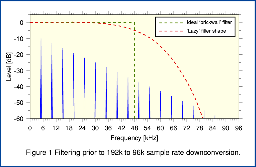
Figure 1 compares two types of filter. For the sake of illustration the graph shows the spectrum of a signal which has a fundamental frequency around 5 kHz and a series of harmonics that extend up beyond 48kHz. The initial recording is at 192k sample/sec.

Conventionally, when wishing to downconvert a 192k sample rate recording to generate a 96k rate version the Sampling Theorem leads us to employ a filter that approaches an ideal of a ‘brick wall’ shape. i.e. All audio frequency components below half the lower sample rate (i.e. below 48kHz in the spectrum) should be preserved and their amplitudes and relative phases/timing left unchanged. However every trace of any components at or above 48kHz in the spectrum should be totally removed without trace. This mathematically ideal filter is represented in Figure 1 by the broken green line. MQA, however, is based on assuming that this is not the best method when it comes to the perceived sound quality of digital audio. Instead what we might call a ‘lazy’ filter is used. This allows through some of the components above 48kHz. So the first stage, conceptually, of the MQA process is to apply a ‘lazy’ filter of a design judged to be satisfactory.

The second stage of the 192k to 96k sample rate MQA encoding method is to then downsample (‘decimate’) the filtered result simply by discarding and passing alternating samples. It is clearer and easier to explain the processes as being carried out in these two stages. But in practice, the processes may be combined if this is convenient, but should perform in the same way.

From the point of view of standard information theory this approach tends to give rise to two problems. The first is that passed components that were above 48kHz in the spectrum now create new ‘aliased’ components in the output. When looking at the result it will appear as if these have been ‘mirror imaged’ about 48kHz or as if the paper the spectrum was printed on has been ‘folded’ along that line. The second problem is that components which are at high frequencies that are below 48kHz will tend to have their amplitudes reduced and may have their relative phases altered. As a result the output waveform and its spectrum will differ from that obtained simply by removing the components at or above 48kHz. In particular, the ’folded back’ components will generally not have a harmonic relationship with the lower frequency components and, conventionally, can be said to represent a form of anharmonic distortion of the resulting signal pattern.

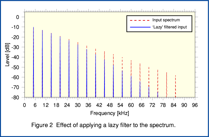
Figure 2, above illustrates the result of applying a lazy filter to the spectrum of a periodic signal contained by the input 192k sample rate series of sample values. From this you can see that the filtered result (solid blue lines) retains components above 48kHz that a conventional filter would seek to remove entirely before downsampling. It also has attenuated signal components in the region below 48kHz. The result is a little like having adjusted an ultrasonic ‘treble control’ to reduce the HF. The MQA patents make clear that this latter effect may well require some treble boost to be applied at later stages in the chain to help correct the change in tonal balance. For the examples on this webpage I have chosen to use a standard ‘Butterworth’ lowpass input filter because its behaviour will be familiar to many electronics and DSP engineers.

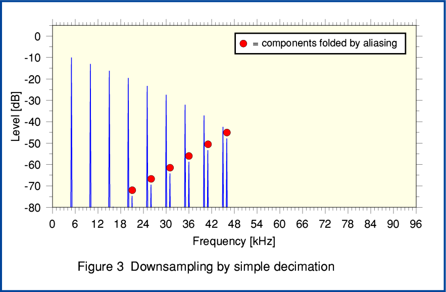
Figure 3, above shows the results when we take the filtered 192k series and perform plain decimation down to generate a 48k rate series for transmission or storage. To make the situation clearer I have added some red blobs to the components which have been ‘flipped’ back by aliasing from the region above 48kHz into the region below 48kHz. You can see that, in general, such components will not have a simple harmonic relationship with the initial set of frequencies. Thus in conventional terms they would be regarded as an unwanted form of anharmonic distortion which is unnatural in nature. Note also that although the levels of these components seem low the output signal would require some HF lift to correct for the input filter rolling down the HF. So when the results are eventually ‘unfolded’ and played the level of these components will be greater than shown here. However the MQA documentation allows for a range of various choices of filters, etc. Hence the details will depend on the choice of filters.

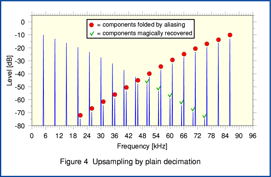
Figure 4 shows what we obtain if we now take the downsampled 96k series and upsample by the simplest method described in the MQA Patent. Here the 48k series are upsampled by multiplying each value by two, and alternating the results with zero padding samples. You can see that this process does – as if magically – ‘unfold’ copies of the components that were aliased during downsampling. Alas it also cheerfully generates unfolded new copies of the original series below 48kHz! If we compare Figure 4 with Figure 2 we can see that this result has many HF components that were absent from the original. In this example these new aliases happen to arise at harmonics of the original series. But note that this won’t be true in general.

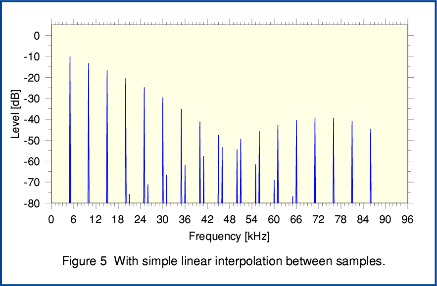
Figure 5, above shows that we can reduce the unwanted aliasing by employing some filtering to the output of the decimation upsampling to 192k rate. Here the filtering is about the simplest possible method – linear interpolation. By comparing Figures 4 and 5 you can see that this does tend to attenuate the highest frequency aliases. This shows that by using a filter after unfolding some of the unwanted aliases can be reduced. The MQA Patent discuss the use of decimation filtering for the downsampling and upsampling. Some specific examples of filter choices are given. These are aimed at correcting the high frequency roll-off produced by the ‘lazy’ downsampling filter, and attenuating the very high frequency portions of the aliasing caused by the upsampling.

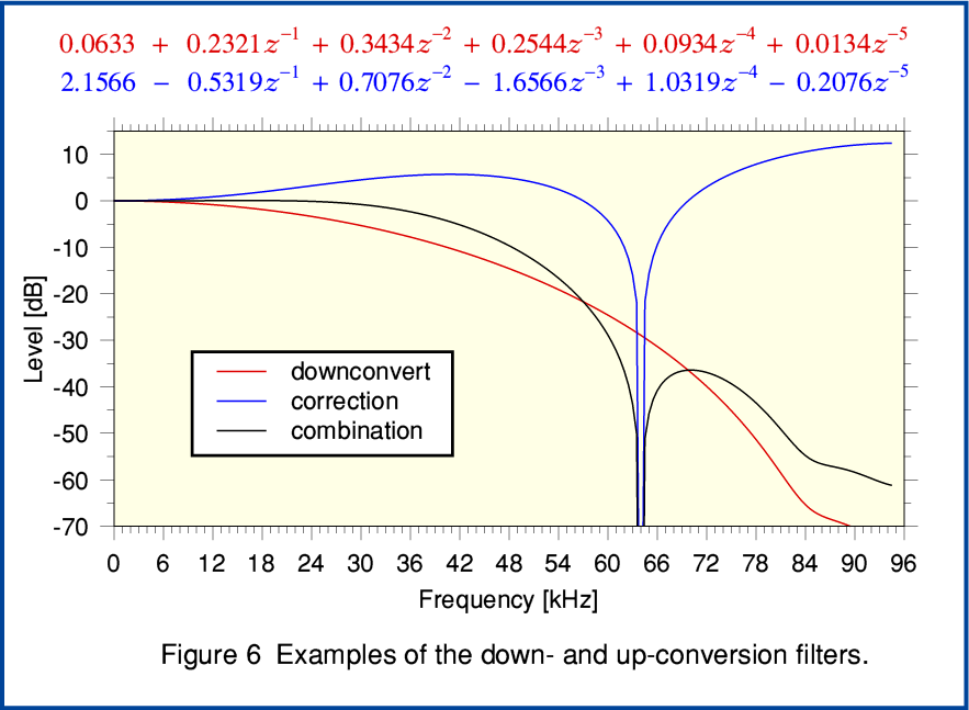
Figure 6 shows a pair of examples specifically defined in the Patents. The solid red line shows the ‘lazy’ downsampling filter. The solid blue line shows the upsampling ‘correction’ filter. The aim is that the combination should give an end-to-end response which is essentially flat up to over 20kHz, maintain a wide enough bandwidth to give a temporal resolution that is sharper than normally possible from conventional 96k rate LPCM, but reduce the higher components arising from the upsampling process. The precise details will vary with the choice of the filters. These can potentially be chosen by an individual creating MQA files or streams as they judge ‘optimum’ for the specific content. Given this, any comments on MQA as a method can only be general ones. However if you compare the plots in figure 6 with those in the earlier graphs some general points can be made.

Firstly, if we wish the ‘origami’ folding and unfolding to give us a sharper temporal response then we must also allow though the aliases over a related frequency range. The more temporal ‘sharpening’ we want, the higher the levels and frequencies we may get from anharmonic aliasing added to the output. We tend to end up with a conflict between making changes to the filtering to get better temporal response versus changes that reduce the amount of unwanted HF aliasing. Optimising this seems to potentially be a matter of the extent to which people with ‘golden ears’ hear aliased components as if they were also part of the musical harmonics rather than unwanted distortion! So it seems to rely on people either not noticing the aliasing (which implies they might not be noticing the HF anyway) or hearing it without being able to notice its actual anharmonic nature in general.

A particular problem can arise from the use of MQA when we wish to consider its performance by doing a listening comparison. We can imagine setting up a test where we carry out an ‘ABC’ comparison. Here ‘A’ would be the original 192k rate file, ‘B’ would be the 96k rate version produced via MQA folding for transmission or storage, and ‘C’ would be the unfolded 192k rate output from ‘unfolding’ ‘B’. Various outcomes may arise from a controlled subjective listening comparison. And the outcome might, in practice, vary from case to case. The difficulty is that both ‘B’ and ‘C’ tend to have added aliases, and that ‘B’ also has a changed spectral balance from having been filtered. Hence we can expect that ‘B’ might sound different to ‘A’ even if a conventional downconversion would have sounded the same as ‘A’!

One particularly interesting outcome is that we might find that ‘A’ and ‘C’ sound different. If this is the case, then it can presumably only be due to some combination of an alteration in the spectral/temporal response of the original components present in ‘A’ with the effect of having added the aliased components into ‘C’ which were absent in ‘A’. The sound of ‘C’ might be preferred to that of ‘A’. If this can occur then we may run the risk of those producing such files sometimes choosing to deliberately alter the chosen filters, etc, to ‘enhance’ the sound. i.e. using MQA as an ‘effect’ rather than a way to preserve fidelity to an original. On the other hand, if ‘A’ and ‘C’ sound the same then it is possible that there wasn’t actually that much audible HF present that needed ‘folding’ in the first place and a conventional downcoversion would also have sounded fine.

Having abandoned keeping to the Sampling Theorem, the results become a matter of subjective opinion, and the creator of the individual MQA file or stream may have some control over this judgement. It then becomes a question of whether each listener likes the result or not. In some ways the creator of an MQA file is placed in the position of being a ‘magician’ who has to know how to get the best sound from an existing recording. Unfortunately, the music business has a mixed track record in such matters. For example, the tendency to equate ‘good’ sound with ‘sells well’ which has led to many Audio CDs being level compressed and clipped to be LOUD on the basis that this ‘sells more CDs’.

However even ignoring the above practical questions there are some more basic or general questions MQA raises. For example: Do we actually need MQA at all? How ‘Authentic’ in audio terms can we regard the results as being given the appearance of aliased components that were not present in the original recording? Are there potential alternatives which can provide provide a similar – or better – level of data compression and deliver good sound quality whilst avoiding the addition of anharmonic aliasing? Thus helping us to preserve a more faithful version of the original whilst squeezing the quart into a pint pot? All being well, I will explore these questions on another webpage...