Combining Low-Pass and High-Pass filters
For crossover or band-splitting purposes we require two (or more!) ‘matched’ filters that neatly divide the signals into the required bands. Ideally without losing, duplicating or boosting any particular bands.
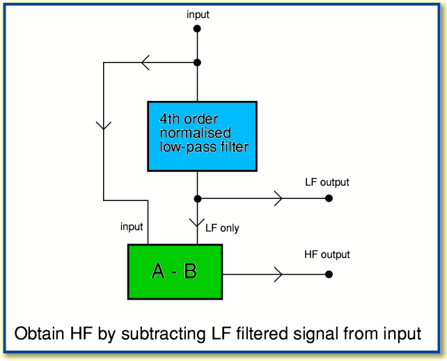
Let us take the example of a filter network or crossover whose task is to divide the signals into bands above and below 1 kHz, but where we wish the vector sum (amplitudes) of the LF and HF outputs to equal the input. We can imagine achieving this quite simply by taking the above 4th order low-pass filter and using it as part of an arrangement as indicated below.
The gain of the normalised low-pass filter is almost unity at low frequencies. Hence if we take the input and subtract the LF output from it, we may expect the result will be almost nothing at low frequencies. However at high frequencies the low-pass filter will have a small gain, so produces very little output. Hence at high frequencies when we subtract the output of the filter from the input we may expect to get the same as the input. i.e. the difference between the input and output of the low pass filter will contain nearly all the high frequency components, but very little of the low frequency components. Hence it will tend to give us a high-pass response.
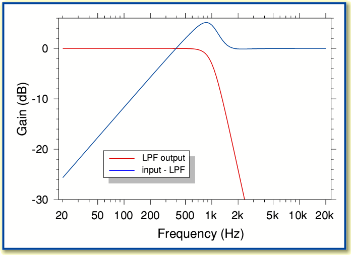
The above graph shows the response this tends to give. Note that the above is normalised on the assumption that the power gain of the LPF is given by  and the balanced HPF output is
  as a result of the subtraction process.
Alas we can see that although the low-pass filtering works nicely (shown in red) the high-pass portion (shown in blue) does not. This arrangement is a poor high-pass filter at it tends not to reject low frequencies very well. It also has an unexpected ‘bump’ in the high-pass output around the nominal crossover frequency region.
The poor low-frequency rejection is due to the gain of the low-pass filter not being exactly unity over the range it tends to pass. Hence we find that the input and low-pass output do not cancel as well as we might wish and the high-pass response obtained by subtraction tends to ‘leak’ more low frequencies than we might like. In this example the high-pass output only rejects signals at 100 Hz by around 12 dB. This is not particularly impressive given that the low-pass filter is 4th order and has a nominal ultimate slope of 24 dB/octave.
In principle the above results may be improved by slight alterations to the filter response. However this means we also have to ensure very tight control over the exact values of components to get improved performance for the high-pass output. As a result it tends to become difficult to achieve good results this way in practice.
The ‘bump’ is actually a sign of a more general problem which we will encounter again if we now move on to ‘better’ arrangements of the kinds more commonly considered for active crossover systems. It occurs as a consequence of the phase effects produced by filters.
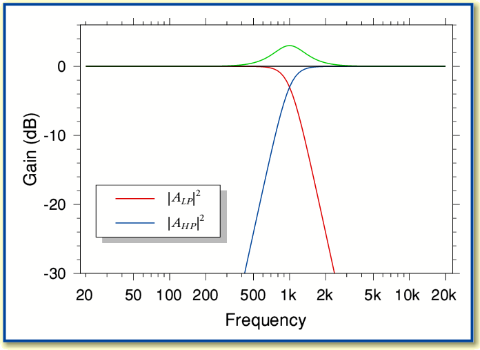
Let’s now consider using a ‘matched pair’ of 4th order filters of the type described earlier. One low-pass, the other high-pass, but sharing the same maximal flat shape, and the same turnover frequency. This will produce the results shown in the graph below.
Here in order to distinguish between the two filters I have indicated the LPF response (red line) with an ‘LP’ subscript and the HPF response (blue line) with an ‘HP’ subscript.
The above graph also shows two other plots. The black line shows a plot of 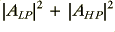 and hence represents the sum of the powers of the two filter outputs. For adding unrelated signals this would give us the uncorrelated (incoherent) result. However when the two filters are driven with the same input their outputs will have a coherent phase relationship. Hence we may then experience their vector summed output. To indicate this the green line shows
 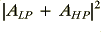 .
.
It is important to note that the green and black lines differ quite markedly in the frequency region around the chosen crossover value (1 kHz in this example). The incoherent power sum shows a flat response, but the coherent vector sum shows a peak. This is because at the crossover frequencies the two power gains (HF and LP) are 1/2, so sum to unity. However the two amplitude gains are only 1/ and add with their phase relationship taken into account.
The effects of the phase and vector addition/subraction is also the reason for the ‘bump’ which appeared when we tried to synthesise an HPF by subtraction earlier. This acts as a warning that when employing such filters for use as loudspeaker crossovers we may have to consider which form of addition is appropriate and act accordingly. Vector addition is appropriate when we wish to determine the on-axis total response of the resulting system. But the power addition may be relevant when considering the total power radiated into a room.
In general, with loudspeakers the preference has been to seek to get the vector sum’s amplitude to be frequency independent. The commonly accepted method for this is to employ the arrangements outlined by Linkwitz in his paper on active crossovers in the Jan/Feb issue of JAES in 1976. The example of a 4th order arrangement in that paper (fig 5) uses Sallen-Key topology, but is equivalent to the circuits used here provided we normalise the gain and select the appropriate damping factor value(s).
For the previous examples we chose different values for  and
and  in order to ensure that the results had maximum flatness with
  still being the -3dB point. However the Linkwitz arrangement is chosen to have the same
  values for both the 2nd order sections of each 4th order filter. This alters the response shape and means the 4th order filter will now have a -6dB point at
  . This represents a significant change from what we considered previously. It is perhaps noting that in general in signal processing electronics the -3dB point tends to be the frequency used to indicate the frequency range a filter is designed to define. But with the Linkwitz 4th order arrangement for loudspeakers it is the -6dB point that is significant as this represents the nominal crossover frequency for this situation.
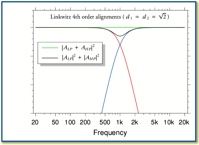
Using 4th order filters the Linkwitz requirements mean altering the damping factor values to be  for all the individual 2nd order stages. In effect, we are now simply using the maximum flatness arrangement for a 2nd order filter we considered initially. If we do this we get results of the kind shown in the plots below.
The vector sum (green line) can be seen now to be flat across the frequency range of interest. We can also see that at the crossover point the two filters now reach -6 dB rather than the -3 dB crossover level we had previously. Note, though, that the incoherently summed power level (black line) now has a dip. Hence we may find that the result has a dip in the total power radiated into the listening room, but the on-axis level in an anechoic situation should, nominally, have a flat frequency response.
In conclusion, the simplest recommendation for an active crossover filter is to employ pairs of 2nd order building blocks with  to construct 4th order low-pass and high pass filters. This means that
  will represent the -6dB point of each 4th order system (-3dB per 2nd order building block) and the responses should crossover at this -6dB point, producing an overall vector sum output which exhibits a flat response. In practice, however, the actual response will depend on the loudspeaker units, so a more complex and specific arrangement may be required to obtain a desired response.
Page 2 of 2
Jim Lesurf
6th Jun 2005