Ringing in arrears?...
The ‘Impulse response’ of a digital system is sometimes shown in reviews of Hi-Fi equipment, etc. Quite often DACs (Digital to Analogue Convertors) include response plots to indicate their behaviour as a reconstruction ‘filter’ when employed to generate an analogue output from a series of digital values from a file or Audio CD. Plots of this kind are useful for engineers because they can be examined to assess and compare the behaviour of DACs and what their output will be like. They have also given rise to it being common for high-quality Audio DACs to offer the user a choice between different reconstruction filters. Alas, a side-effect of this is that they have also become widely misunderstood or misrepresented in discussions about domestic audio. As a result some myths have arisen. Most recently, the MQA system has reportedly adopted a quite specific stance on this issue which may also be based on a combination of a misunderstanding and considering them out of context.
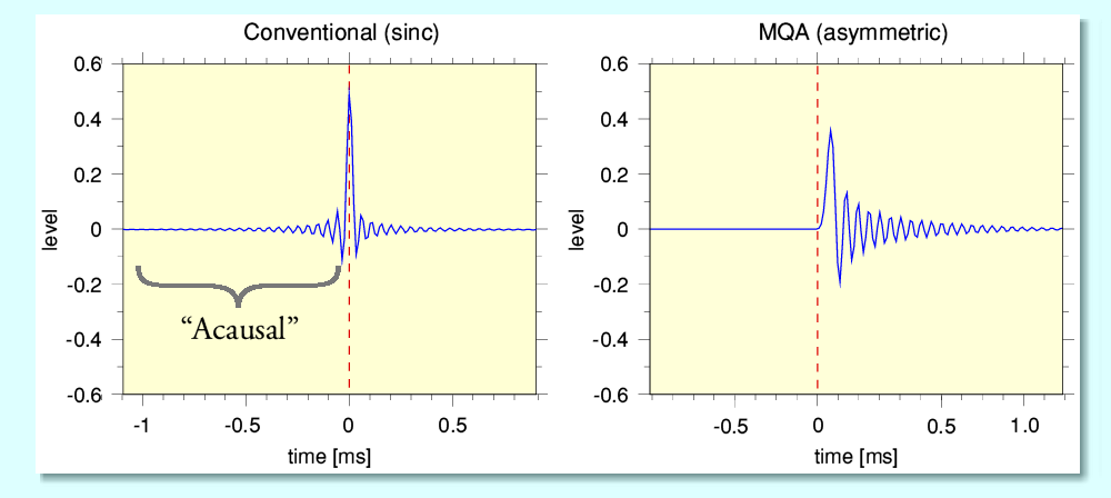
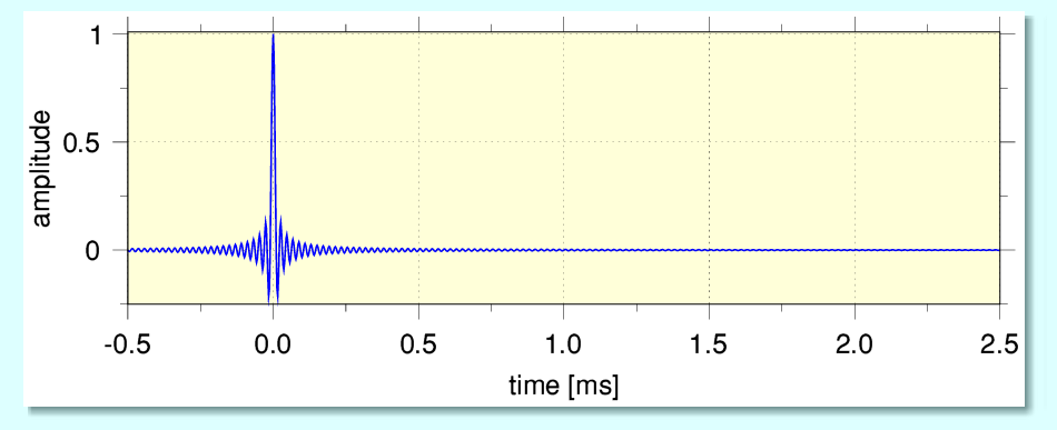
The above plots illustrate a key difference between categories of impulse response. In each case they were prompted by an initial single isolated non-zero sample value surrounded by zero values. i.e. a digital ‘impulse’. (The broken red line has been added to indicate the instant when the non-zero impulse was encountered.) This form of digital test signal is often used to ‘read out’ the impulse response of a DAC. These patterns can be then also transformed to produce the frequency response of the DAC’s reconstruction filter.
The above graphs show different impulse responses to the same set of LPCM information. The ‘Conventional’ response was obtained using a reconstruction filter based on a sinc-function of the type specified by the basic tenets of Information Theory[1]. The asymmetric response was generated when the source material was played with an MQA DAC decoding the same data. This is claimed to ‘sound better’. In addition various assertions have been made to the effect that the conventional form of reconstruction must be flawed because the ‘ringing’ which seems to arise before the arrival of the input impulse must be “Acausal”. i.e. we see the response before the stimulus that generates it – a violation of causality! The asymmetric response removes this obviously incorrect behaviour and is therefore more ‘natural’. However things are not as that may seem...
Jim’s Law
“Data only becomes Information when you know exactly how it was obtained and processed.”
The above statement is one I adopted as a maxim some years ago. This was partly a result of teaching undergraduates Information Theory and how it could be applied. When doing this I realised how often people fell into the trap of incorrectly assuming the terms ‘Data’ and ‘Information’ are synonyms. It also came from working on developing and using novel instruments to collect data in order to yield new information. Given how often I’ve had to quote it, I’ve come to call it “Jim’s Law”, but despite that I simply regard it as something that should be obvious once you understand how to apply the basics of Information Theory.
When we come to consider the behaviour of a DAC we wish to use to convert a stream of digital data into analogue waveforms Jim’s Law means we need to be clear how that stream of digital data was produced from an original source. The proponents of MQA apparently say that an important part of their process is to ‘deblur’ (their term) the effects of the ADC used to record the audio. This is then apparently given as one of the reasons the MQA system tends to output an asymmetric impulse response. The assumption being that this ‘corrects’ the behaviour of the original ADCs used to make a digital recording by removing the ‘acausal’ pre-ringing. Unfortunately, this argument is flawed on more than one level! To see why we need to apply Jim’s Law to the recording process that produced the digital data which might need such ’correction’.
The critical point here is that that an ADC is NOT the start of the process. Before the ADC comes an – often very complex – set of previous processes. Many recordings were made using a number of different microphones, electronic sources, etc, etc. All feeding though various mixing/modifying stages. Quite often different parts being recorded at different times though different arrangements. The result then gets ‘mixed down’ to stereo and may have been though various digital and analogue pathways on its journey to that stereo result. Even the simplest recordings of acoustical sounds will tend to have a number of stages.
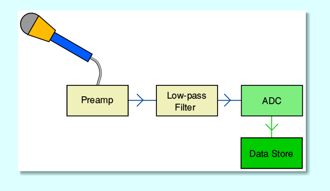
The above represents one of the simplest arrangements we can consider. It starts with a single microphone to detect the original acoustic sound. It converts the sound pressure variations at the microphone location into an analogue signal whose voltage varies with time in a way related to the detected sound pressure. This output is amplified to give an electronic signal at a higher level. One of the basic requirements for digital audio is to ensure we can avoid ‘aliasing’. This can arise when the analogue signal pattern contains frequency components at frequencies that are equal to, or above, half the sampling rate. To deal with this an analogue low-pass filter may be employed for the signal to pass though before it reaches the actual ADC stage. The ADC then converts the (filtered) analogue input it is given into digital data and this is stored as a recording.
Each part of this process will have its own limitations and potential effects on the information passing though them. To fully determine the real information content and meaning of the recorded digital data we would need to take all their effects into account. Here, though, I will simply consider the microphone to serve as an illustration of the way this can affect how we interpret the data which is recorded.
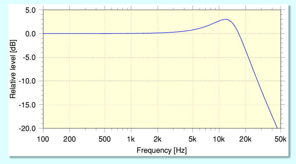
Many microphones used for recording music have a frequency response which is far from being flat across the frequency range from below 100 Hz up to well over 20 kHz. The response varies from one model to another. Indeed, as a result some recording artists or producers have tended to like to choose specific microphones because they give the ‘sound’ they prefer. In addition, the response tends to varies with distance from sound source to mic, with the angle of incidence, and even with temperature! Many widely used microphones have a ‘ring and die’ high-frequency response. i.e. they show a clear resonant peak in the region somewhere above 10kHz, and above that the response dies away rapidly with increasing frequency.
For the sake of simplicity I’ve represented this with the above plot of sensitivity versus frequency showing a sort-of-typical behaviour. The phase/time behaviour of the microphone’s audio response will also vary with frequency in a way that is related to the gain/frequency response. In essence we can regard the microphone as a transducer that has the response of a simple 2nd-order low-pass filter. If we then assume we can find a sound source that will generate a perfect sound pressure impulse we can calculate the resulting impulse response output by such a microphone.
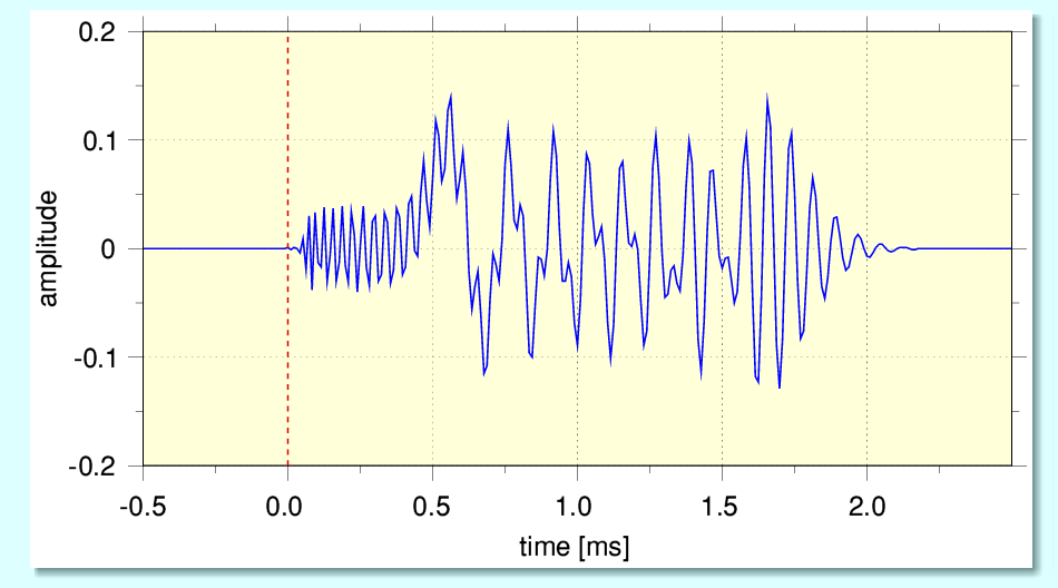
The above shows the resulting impulse response from our simple microphone, assuming the recorded spectrum will reach to 48kHz (i.e. 96k sample rate). The broken red line shows the nominal instant when the sound impulse hit the microphone.
Note, however that real microphones tend to vary and are often more complex. However two basic points can be seen from the above:
Even if the following preamplifier and any inserted low-pass filter are perfect, this is what the ADC will get – NOT an impulse! Hence what reaches the ADC is already spread out across a time-period after the nominal input impulse instant. And is actually spread out over a wider period than the ‘correction’ which MQA seems to apply regardless!
In an ideal world we would be able to choose to employ a microphone, low pass filter, and ADC which all had a perfectly uniform amplitude and time-delay response up to 48kHz when making a 96k rate recording. Such a system would then give an impulse response as shown above. Although this exhibits the often-scorned ‘pre-ringing’ we can see that in terms of time-alignment and avoiding dispersion it is dramatically better than a typical microphone and would do a much better job of preserving the details of fast transients. And in practice well designed digital components like an ADC tend to do rather better in these terms than analogue filters that may precede them, and significantly better than most real microphones, etc, used in studios over the decades.
In addition, the variations from one microphone to another, their behaviour varying with temperature, angle of incidence of sound, distance/proximity, etc, mean that the changes made to the signals before they reach the ADC tend to be complex, variable, and probably impossible to completely unscramble after the event.
As a result, the general implication is clear enough: In practice it makes little sense assume we need to ‘correct’ for ADC pre-ringing or force the eventual stereo DAC to apply a blanket ‘correction’ for the ADCs employed during recording. Indeed, doing so seems to ignore the real elephants in the room – e.g. the microphones where the electronic signal path begins. It also neglects later stages in the path to an eventual stereo mixdown release including ignoring any ‘EQ’ that was applied by those making the recording before the signal reached the ADC. For older recordings we can add in the effects of mixing desks, analogue tape recording, etc. Given all these variables worrying about the ADC seems more like a displacement activity than a sensible course of action!
The other end of the telescope.
Having made the above point we can ask a question which looks at this topic from the other end of the signal path: “What would we have to put into an ADC in order to get out from it the test signal that Hi-Fi reviewers and pundits normally use and call an ‘impulse’ when assessing a DAC or digital data convertor?”
Given a chosen sample rate, Information Theory requires us to ensure that sampling obeys the Nyquist requirement and prevent any frequency components that are not below half the sample rate from being sampled by the ADC. Failing to do this will generate aliased components in the sampled data that weren’t in the input signal. i.e. add distortion.
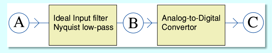
The above diagram shows the vital functions that an ADC needs to perform. Here, and in what follows I’ll assume for the sake of example that we wish to sample the audio at 96k samples/second. And I’ll just consider one channel and assume we could simply operate a set of these in parallel for stereo or multichannel conversions. I’ve also divided the process into distinct sections and assumed we choose to use an ideal analogue input filter which then feeds the actual ADC. This makes explaining the essence of the process easier. But in practice the two functions may be combined and, for example, some of the input filtering may be done by a digital low-pass filter. The ‘A’, ‘B’, and ‘C’ in the diagram represent: the signals we put in (‘A’), what this then generates after the input filter (‘B’), and the resulting series of samples (‘C’).
The ideal performance for an input filter used before an ADC is that is should pass all frequency components up to the Nyquist frequency (48kHz in the case of our example) without altering their relative amplitudes or phases and it should totally block any input at frequencies equal to or above 48kHz. This means that the wanted spectrum is passed on, unaltered, whilst preventing any input that would generate aliasing distortion from reaching the actual ADC.
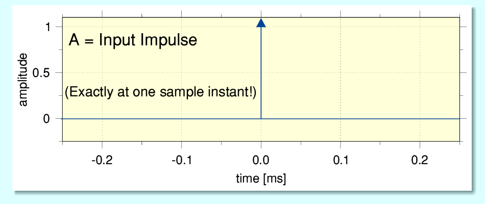
The above illustrates presenting an input, ‘A’, that consists of an essentially perfect impulse function. Note that I have put an arrowhead on the impulse to indicate that it is has a much higher peak amplitude – in fact should have a nominally infinite amplitude for a perfect impulse! In reality, of course, that is essentially impossible to achieve but we can assume that we could generate an input that is close enough to seem like an impulse when we only consider its components up to 48kHz because out first process is to block anything above that frequency. In practice, of course, even getting this from real audio recordings of music is unlikely given what we’ve already seen about the behaviour of microphones and other real-studio items! Note that here I also use a timescale that is set so that the time equals zero at the instant of the impulse at each stage in the chain.
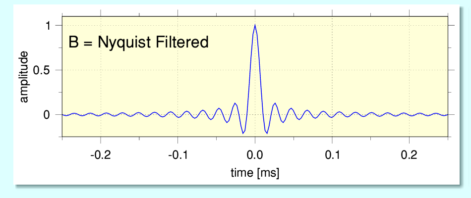
The above shows the result we get at ‘B’ having passed the impulse though our ideal low-pass filter. This has the standard textbook ‘sinc function’ shape. This is the case because the time-alignement of all the passed-on frequency components are maintained to be in-phase at the nominal instant of the impulse. Hence we get the textbook symmetric shape that concerns some reviewers and audiophiles and gets labelled ‘acausal’. The implication being that this must be wrong in some way. However if we pass this on to the actually sampling process we can get out...
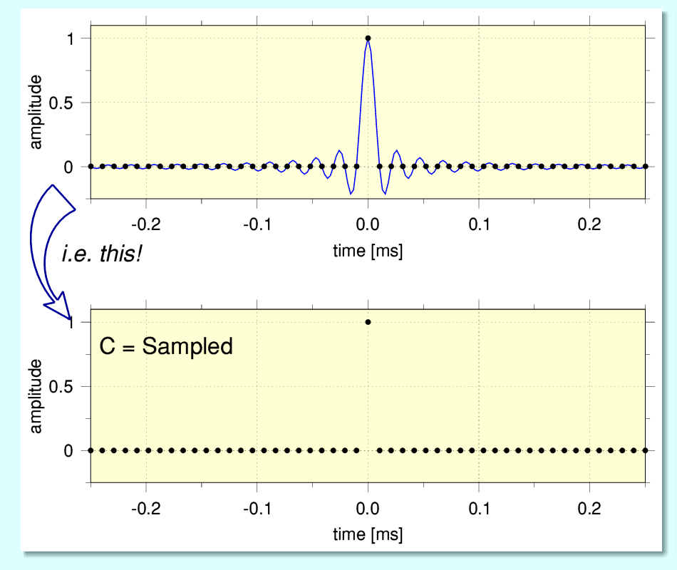
...the result ‘C’ shown above. Here the time when the impulse reaches the ADC conversion corresponds with one of the sampled instants. The result is a single non-zero sample regardless of the extended sinc pattern! This is because the sinc shape neatly goes though a zero-value at all the other sampled instants.
From the above we can see that it is, indeed, potentially possible for an ADC system to capture an impulse and record it as a single isolated non-zero sample value. However the requirements are quite specific and very demanding. In particular, the input impulse has to hit a sampled instant on the nail and we need an amazingly good input filter! Indeed, we need one that converts an input impulse into a sinc pattern. This neat result raises some questions – e.g. what about coping with an input impulse whose arrival time does not neatly coincide with a sampled instant? However before trying to answer such questions I’ll look at what happens when we want to regenerate the above digital output with a suitable DAC arrangement.
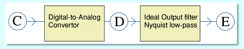
The above represents the way the stream of digital values can be converted back into an analogue waveform. The output filter has the same behaviour as the input filter. It passes all the components up to the Nyqist frequency whilst preserving their relative amplitudes and phases, but entirely removes anything at or above the Nyquist frequency.
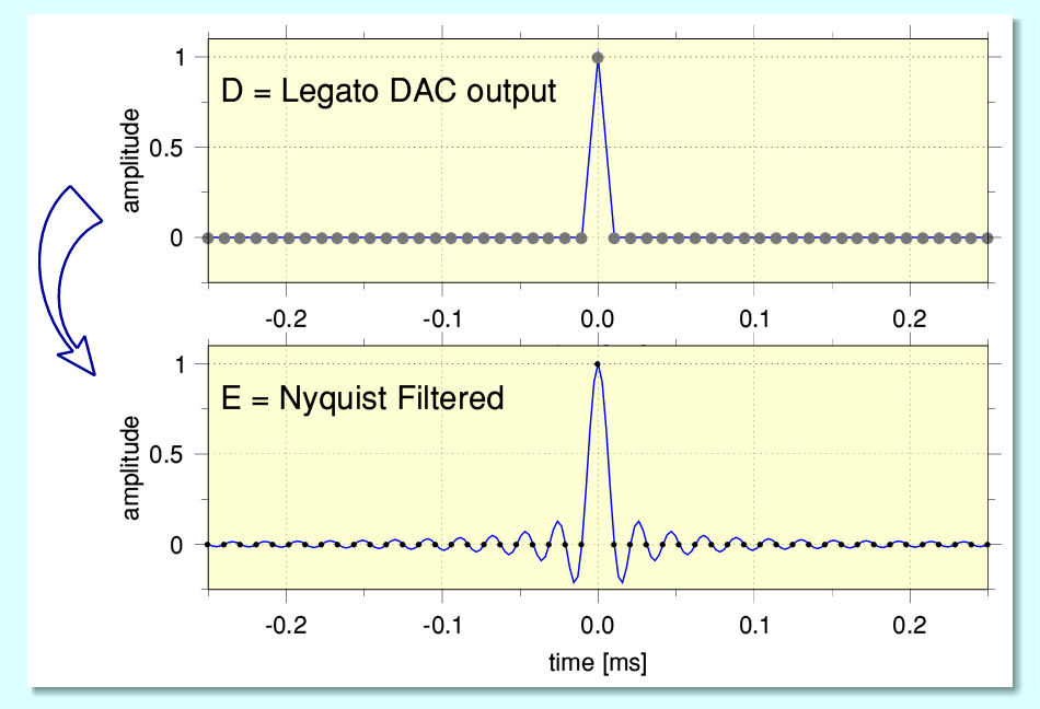
The above shows what we then obtain as the analogue output. For the sake of example I assume the DAC adopts what Pioneer called a ‘Legato Link’ method which creates a waveform that ‘joins the dots’ with straight lines. Various other approaches exist. e.g. ‘sample and hold’ which generates a rectangular profile in between each sample and its successor. Alas, all these simple shapes tend to create distortion components and require extra filtering. (‘Sample and hold’ also delays the output by half a sample interval.) The good news is that when we run this DAC output though an ideal Nyquist filter we get the result shown as ‘E’. This matches ‘B’ exactly! (I’ve included the dots showing the sample instants for the sake of comparison.) Hence – so far as the signal information below the Nyquist frequency is concerned – the output matches the input. Various techniques can be employed to carry out these processes, but should in principle be able to replicate the above behaviour.
The obvious question now becomes: What happens when the input impulse is not neatly aligned with a sample instant? To answer this question we can consider a situation where the impulse arrives half way between two sample instants. One potential problem then becomes clear: If we’d simply decided not to use any input low-pass filter at all before the ADC we could find that the impulse simply failed to be noticed at all! Generalising from that we would get the result that the presence of components above Nyquist would tend to seriously muddle the recording with added distortion products due to aliasing. The good news is that by ensuring we employ a suitable input filter before the ADC we can avoid these problems. So we should stick with a filter like the one we have adopted above.
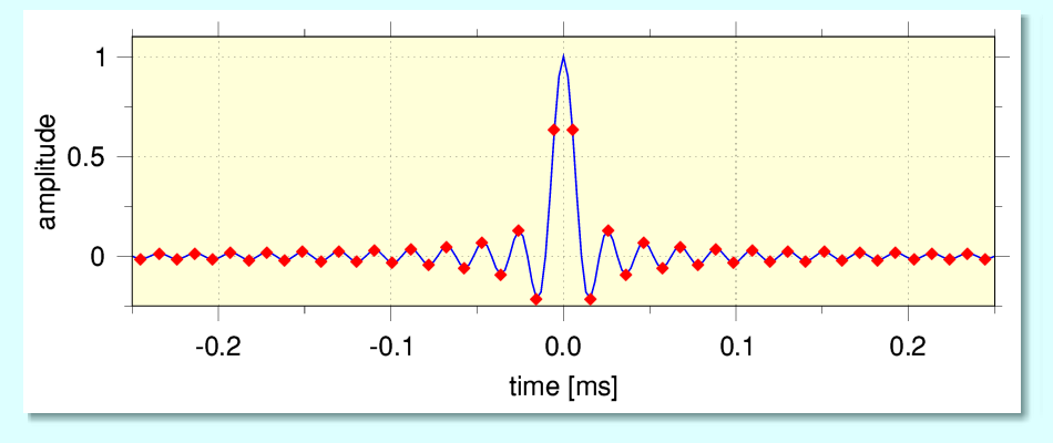
The above illustrates what we would obtain in this situation using the system described above. (Note that time axis is still shown relative to the time of arrival of the impulse. And that I have left the samples visible so you can see where they occurred relative to the impulse.) Now that the input impulse is midway between sampled instants we can see that the actual sample values no longer emerge as a single non-zero value surrounded by zeros. Instead, the samples ‘trace out’ the sinc pattern explicitly. This means we don’t get the neat ‘one sample’ pattern beloved by reviewers. However when we then play this series though our DAC and its filter we get out a sinc pattern with its peak at the correct time, mid-way between samples.
This shows that – although we can use a time-aligned impulse as a ‘special case’ and use a single non-zero value for tests – more generally the use of this type of filter means that we get the same kind of output regardless of the actual instant relative to the samples of the impulse. We can represent any impulse correctly whenever it occurred during the process of a recording including accurately indicating its time of arrival. For any arrival instant the output waveform has the same shape and spectrum, and appears with its peak at the appropriate instant. We got out the same pattern as was presented to the actual ADC.
You pre-rang, Sir?...
So why isn’t ‘pre-ringing’ to be shunned as an un-natural and even ‘acausal’ behaviour, implying it must be un-natural?
Well, one part of the answer to that question surfaced earlier in this examination. When we start off with real microphones capturing real audio, they generally give a response from an impulse that lacks pre-ringing. And when we look at musical instruments like electric guitars we will tend to find similar behaviour. Twanging a string and having that sensed with a pickup also tends to act in similar way. Similarly, pounding a piano key to hammer a note from a piano doesn’t actually generate a transient that is infinitely steep. The hammer and the string have finite elasticities. It takes time for the impact deformation under the hammer to rise, and for this to start propagating along the string, etc. The processes are very fast, but you don’t get a mathematical impulse or step-function. The sound pressure radiated takes a finite time to rise.
At this point we can also consider how a simple old-fashioned analogue filter works. In general to make such a filter you’ll need to make a circuit that contains at least one capacitor or inductor. The more complex the filter may be – and the closer it’s behaviour gets to the ‘brick wall’ Nyquist ideal – the more capacitors and/or inductors it will need to employ. In a similar way, digital filters tend to require more memory locations, etc, to approach a ‘brick wall’ response.
Usually, electronics books discuss this in terms of the ‘order’ of a filter. But more generally in mathematical terms this can also be regarded as the number of relevant ‘variables’ or ‘dimensions’ it has. The voltage on each capacitor and the current passing though each inductor at any instant represents the ‘state’ of the filter at that instant. And that state has been generated by the pattern of the signal which has been fed into it over a period of time up to that instant. i.e. The filter has a ‘memory’ which causes its behaviour now - and for a while to come - to depend on what input signals it has seen ‘recently’. This, in turn, means that it will tend to delay signals passing though it.
If you follow though the mathematical implications of this you find that filters of the kind we require have to employ a distinct time delay between when we input a signal, and when the matching output emerges. As a result, pre-ringing isn’t actually ‘acausal’ it is just a feature of the nature of the relevant kind of signals and filters. In practice, of course, real filters can only approximate to a perfect Nyquist performance. One aspect of this is that they tend to employ an ‘apodised’ filter which replaces the sinc pattern with an approximation whose impulse response fades to zero over a finite time period. That then tends to set the time delay imposed for signals to pass though the filter. But the actual frequency components may remain well time-aligned despite the ‘pre-ringing’ shown by ideal impulses obtained on a test bench.
Real mechanical systems can also temporarily store energy. This is why microphones lack an ideal impulse response. And the same is true for loudspeakers...
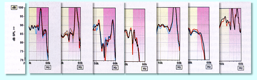
The above shows a section of the frequency responses from a series of loudspeaker reviews that I chose at random. I’ve only included the sections from 10kHz to 60kHz. (If you subscribe to Hi-Fi News magazine you can probably look through your back issues and identify the loudspeakers. But here their identity doesn’t matter here, just the behaviours they tend to exhibit.)
They are all high quality speakers that deliver excellent sound quality. But the variations in performance above 20kHz are quite stark! In some cases they show an HF resonance that reaches more than 10dB above the overall level below 20kHz. Indeed, in one case a resonance above 20kHz resonance reaches almost +20dB! And in another case there are two quite sharp and distinct resonances. These peaks tend to arise as a result of tweeter ‘breakup’ where the radiating part of the speaker ceases moving in a uniform manner. The result also tends to be highly nonlinear in many cases. One consequence of this behaviour is that it degrades the impulse response and adds more time dispersion.
In addition, most high-quality loudspeakers actually employ two or more drive units and split the audio into frequency bands to drive them. This behaviour, along with cabinet resonances, also tends to change the impulse response and add more time dispersion. So – as with microphones – we may find that even well-regarded loudspeakers can affect the impulse response in a way that may swamp any concerns about the ADCs used to make a recording or ‘pre-ringing’.
Taking all these real-world factors into account we can generally conclude that the appearance of sinc-like pre-ringing in lab-bench tests may simply be confirming that an ADC or DAC is working as they should. Correcting for the microphones used for a recording might in principle make more sense – if our loudspeakers and listening room acoustics were blameless.
That said, in practice correcting this much later on is virtually impossible because microphone response varies with distance to the sound source, angle of incidence, etc. And quite often the microphones were chosen and placed to use the mic to give a preferred ‘sound’ anyway. One which would have spread out the impulse response response ‘to taste’ – before it went though the mixing board and other modifications applied by the recording engineers. Older recordings that were originally made onto analogue tape will also have been altered by that process as well. Anyone who is familiar, for example, with the old ‘Dolby A’ analogue recorders might feel an urge to tear out their hair if they want to ‘correct’ a resulting recording’s temporal response behaviour as the frequency-banded levels pump up and down...
Overall, when we take into account the various other factors involved in audio my own general conclusion about MQA’s apparent concern with ADC ‘correction’ is much that same as my view of other aspects of the MQA process. It can be summed up as probably being “Mostly Quite ’Armless”2[2]. i.e. the ADC ‘correction’ they make seems to be modest compared to what happens at other stages. So in practice it probably an irrelevance that doesn’t matter much one way or another. More about marketing than music.
If the source material was good, then the MQA’d result probably will also sound good. The main snag for listeners will be, however, that if MQA prevent people from also listening to what went into the MQA process they will be unable to actually tell what – if any! – audible change ‘correcting’ for the ADC may have made. So unable to make a fully informed choice. However in practice the only impact may be the added cost to fund MQA when – given a chance – the listener might have been just as happy to get a version that bypassed this entirely.
Jim Lesurf
4200 Words
20th Jul 2021
[1] See, for example, chapter 7 of http://jcgl.orpheusweb.co.uk/InformationAndMeasurement_PDF_Book_pf.pdf
[2] More on that here: http://www.audiomisc.co.uk/MQA/investigated/MostlyQuiteHarmless.html