MQA and “Bit-Stacking”
MQA has a number of different aspects and facets. One of its main stated aims is to achieve a reduction in the size of the files and streams required for conveying “high rez” audio. I’ve seen two basic sets of patents dealing with two quite different MQA methods for this. One ‘folds’ some of the high frequency information back into the baseband when downsampling to a lower rate. It can then ‘unfold’ the result upon replay. I have already examined this “origami” technique on a previous webpage.
Here I want to look at the second MQA technique. For the sake of convenience I’ll call this “bit stacking” as the term may help people to understand how the process works. This will also help to make clear that the resulting arrangements of bits per sample are not quite the same as plain, conventional LPCM (Linear Pulse Code Modulation), although they may be played as if they were. By using a distinct term it becomes easier to distinguish these stacks from plain LPCM samples when it comes to interpreting the meaning and the properties of the sets of associated bits involved.
Judging from the examples in the relevant MQA patents, the origami method is mainly aimed at conversions between high resolution sample rates. e.g. conversions between 196k and 96k. Bit stacking seems to be intended mainly for conversions that are made to create material at the lower sample rates of 48k or 44.1k for transmission and storage. Here, ‘transmission’ may mean in the form of a file for downloading and storage, or an internet stream, or via a physical CD, etc. As with the origami examples, the resulting lower rate files can be played, and music heard, even if the player doesn’t know how to unravel the MQA ‘extras’.
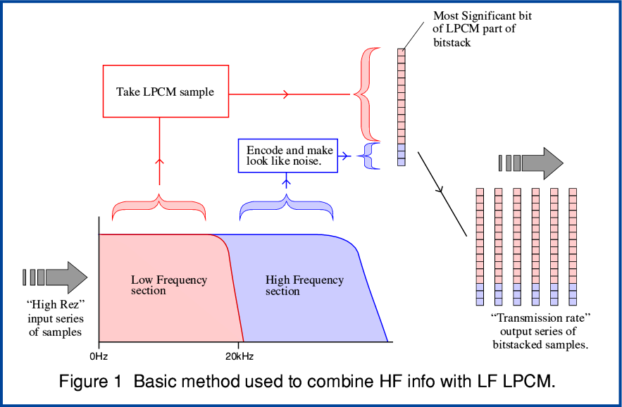
Conceptually, a simple form of the bit-stacking method can operate as illustrated in Figure 1. I will deal with more detailed specific examples later. These have some added complications, but before getting to those, a basic example should help to clarify what is being done.
For the sake of example, consider a situation where the input is LPCM at a 96k sample rate and we want to MQA convert this down to an output at 48k sample rate. Traditional downconversions would just resample from 96k to 48k using a filter that approaches the Nyquist ideal of a low-pass “brick wall”. i.e. This would be designed to try and pass all the spectral components below 24kHz without altering their amplitudes or phases, but remove all trace of any spectral components at higher frequencies. In effect, only information in the ‘LF’ (Low Frequency) part of the spectrum would get though. Any ‘HF’ (High Frequency) audio would be lost and no sign of it would appear in the resulting output 48k rate LPCM. This 48k series of LPCM samples would then convey the transmitted information.
The MQA process alters the situation by reserving what would normally be the least significant bits of the output LPCM and using them, instead, for an encoded series of bits that represent information about the HF part of the spectrum which didn’t get though an LPCM downconversion of the LF region up to 24 kHz. The result ‘stacks’ the combination with the LF LPCM using the most significant bits and the – MQA encoded – HF info occupying what would otherwise have been the least significant bits of the LF PCM. The term ‘bitstack’ acts a reminder here that the result has a hybrid nature which requires special processing to fully and correctly interpret. The information in the bottom bits of each bitstack is encoded in a different way to the information in the upper bits. This matters because in Information Theory we need to know exactly how data (bits) were created to then be able to correctly interpret them and recover all the contained information. Data only reliably conveys information when we know, unambiguously and correctly, how to read it.
The aim is that conventional (or ‘legacy’ players as described in the MQA patents) can now play the result as if it were plain LPCM and – provided the HF info is suitably encoded - simply react to the HF in the least significant bits as background noise. Information is ‘lost’ so far as a conventional player is concerned, but its misunderstandings regarding the meaning of the least significant bits should manifest as extra noise.
The hope is that this extra noise isn’t a concern for listeners using ‘legacy’ players for reasons which I’ll discuss later on. However the same output can be read and interpreted by MQA-capable players which understand how to recover the added HF info. These can then reproduce audio with a wider bandwidth than would be conventionally possible for a 48k rate pure LPCM stream because they know how to fully and correctly interpret all the data (bits). The advantage is that the output bitstacks are at a reduced sample rate, 48k, instead of the input 96k. So the total number of bits per second required to carry the audio information can be reduced.
In principle this is an elegant and neat way to pack a wider bandwidth into the transmitted output whilst retaining some compatibility with plain LPCM replay. However any devils will be in the details. To delve deeper we can now look at two specific examples of the use of this approach, which I will base on ones described in the MQA patent WO2013/186561. As with the previous Patent described processes for “audio origami” bear in mind that what is described are possible ‘examples’ and hence any specific real MQA system may differ in detail. The examples are just a guide to the general behaviour.
96k into 48k/24
This example is assumed to be aimed at streaming or file downloading where the use of 96k sample rate and its multiples are common for high rez material, and that the individual MQA processed output bitstacks will be 24bit at a 48k rate.
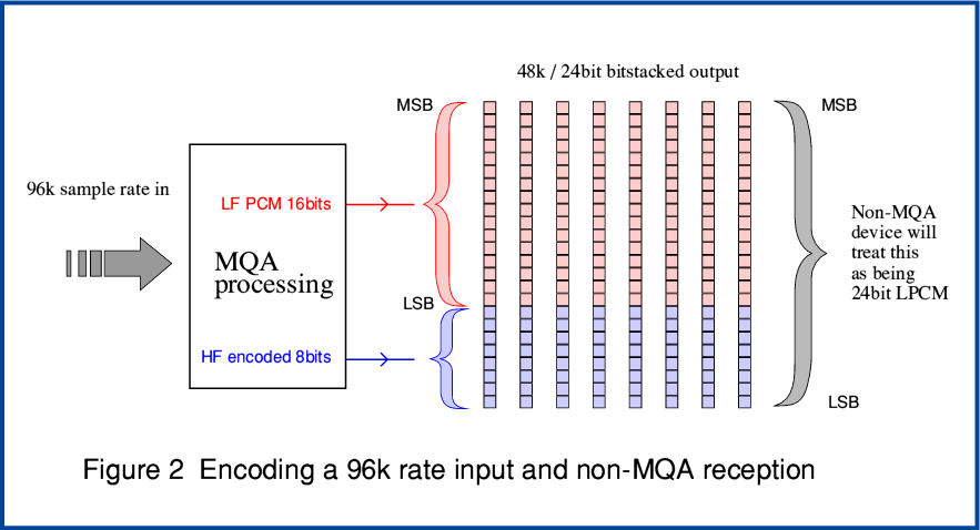
Figure 2 represents a situation where an input 96k sample rate LPCM stream is MQA processed down into a 48k rate series of 24bit bitstacks. The low-frequency information is placed in the top 16 bits of the stacks. It essentially represents a 16 bit stream of LPCM if considered in isolation. The extra MQA encoded information about the HF part of the spectrum is encoded into the bottom 8 bits of each stack. These bitstacks may then be placed in a file or streamed just as if they were plain 24bit LPCM samples. For example, stored in conventional containers like a 48k/24 Wave file.
An MQA capable player can recognise that the information is a series of MQA bitstacks and proceed to recover the added details encoded in what would otherwise be the least significant 8 bits of each sample. Hence it can reconstruct an output that covers a signal bandwidth that is wider than the 24 kHz upper limit conventionally imposed on a 48k sample rate stream. A player which can’t correctly recognise and interpret the MQA HF information at the bottom of the stacks will treat the bitstacks as a 24bit LPCM series of LPCM sample values.
However the MQA system seeks to process the HF into a pattern which – when played on non-MQA players – will behave in a similar way to random background noise. When this succeeds the result will, upon conventional LPCM replay, seem like noise at a levels just under -90dBFS. In practice this should mean that anyone playing the bitstacks as plain LPCM will get essentially the same kind of output they would obtain from playing 48k/16bit LPCM material. Whereas anyone paying the bitstacks using a system that can decode MQA will get an improved result in terms of audio bandwidth, etc.
From the previous webpage on the ‘origami’ MQA method we can see how that can, for example, halve the raw data rates required by folding a 192k/24bit LPCM series of LPCM into a 96k/24 series. i.e. halving the LPCM rate and thus the size of any LPCM file or stream. The bitstacking technique as described above could take, say, an input 96k/24 stream and process it down into a 48k/24 bitstack stream whose values could be stored just like LPCM. So by combining the two we might see a reduction factor of four in the size of the required number of bits we need to store or transmit. In essence this forms the basis of the argument that MQA is desirable as a way to get high resolution audio quality into smaller streams or files.
However all the MQA methods I have considered here and on the previous page omit from consideration the application of existing lossless methods like FLAC, ALAC, or WavePac. So we need to keep in mind that to fully assess this we would have to bring these methods into consideration if our concern is to reduce the sizes of files or streams. This is something I will do, but on another webpage that deals with some of the wider issues associated with MQA.
88·2k onto CD
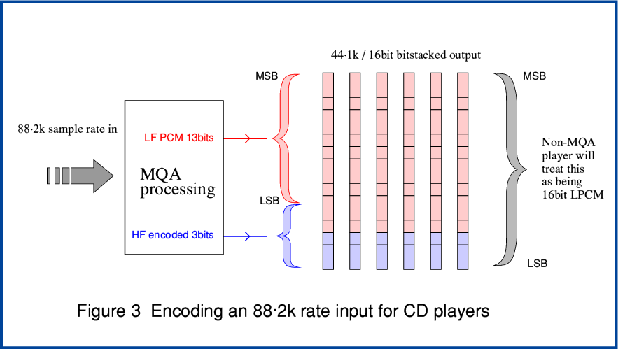
The second example I can use to illustrate MQA bitstacking is one the patent outlines for use for data that may be written onto CDs that may be played on Audio CD players. Figure 3 shows an example of this. Unlike the earlier example, data intended to be used on such CDs is limited to 16bits per sample value. This means that to find space to put the MQA encoded HF details at the bottom of the bitstacks the system has to allocate the LF LPCM less than 16 bits per sample. The example in the Patents allocates just 13 bits per sample for the LF LPCM, and takes the bottom three bits per sample for the MQA encoded HF details. The consequence of this may be to reduce the precision of each individual LF LPCM sample by a factor of eight. So in practical terms the obvious concern is that this implies a reduction in the available dynamic range and a potential rise in the noise floor level of around 18dB compared with plain 16bit LPCM when the bitstacks are used with a standard Audio CD playing system that regards them as being 16bit LPCM.
To try and ameliorate this deterioration the MQA Patents suggest that the LF LPCM section should be noise shaped against the HF encoded lower portion’s apparent value when treated as part of a 16bit LPCM. Noise Shaping is a familiar technique to digital audio engineers when they want to process a digital signal. For the general public perhaps the most widely known example of the method is Sony’s Super Bit Mapping (SBM). But this is just one specific proprietary example of a well-established general method.
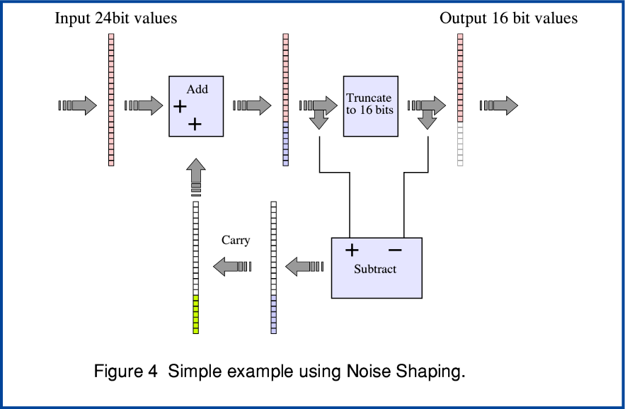
If we ignore for a moment the MQA process as such we can use a simple example to see how Noise Shaping works. Figure 4, above, illustrates how it can be employed when downsampling from a 24 bit input series of LPCM sample to an output series at the same rate that only has 16bits per sample. Bear in mind that Noise Shaping can be performed in various ways, but that here I have chosen one of the simplest techniques to make it easier to follow.
The essence of Noise Shaping is that we ‘carry over’ any details that otherwise might be lost during a resampling or requantisation. In this example when we truncate a 24bit value to a 16bit value we remove the contribution of its least significant 8 bits. But we can then subtract the truncated result from the original 24bit version to retain these ‘lost’ bits. We can then add this retained value to the next value in the input series of values. This means the details aren’t totally lost and can make a contribution via later samples. This process works remarkably well when the sample values are changing relatively slowly as the buildup of ‘carried over’ amounts rises and eventually passes though the truncation. As a result, for audio components which are at frequencies well below half the sample rate the end result is a pattern which is actually more precise overall than the individual 16 bits output samples!
In general, careful resampling or requantisation to a lower sample rate tends to add what is often called “quantisation noise”. Noise Shaping has the effect of altering the spectrum of this noise. The tendency is that noise becomes spectrally ‘shaped’ with a most of the noise being at high audio frequencies. Fortunately, human hearing is less sensitive at these higher frequencies. Hence the name “Noise Shaping”. In fact, the variations here aren’t truly ‘noise’ but an artefact of the processing which exhibits some characteristics of genuine random noise. Overall, the process doesn't reduce the actual total amount of noise. But it can shift a lot of it away from the frequencies where our ears are most sensitive.
Having explained the basic idea of Noise Shaping we can now look at its application to MQA.
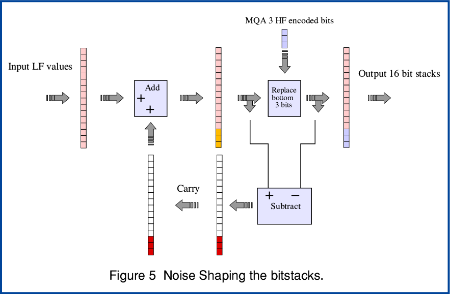
In the case of the MQA reduction of the LF PCM down to 13 bits the Noise Shaping subtraction process would take the difference between an initial 16bit LF value and the value once its smallest three bits are replaced by MQA encoded HF data. In effect, the process assesses how a conventional 16bit LPCM player would respond to the output bitstack and applies noise shaping to try and turn any errors it thus makes into high frequency ‘noise’. As a result, the MQA Patents (e.g. WO2013/186561) say that this shaping can allow the replay using a conventional LPCM player to achieve results equivalent to plain 16bit LPCM for audio spectrum components in the region around 5 kHz or below. i.e. where human hearing is most sensitive. The Patent documents give various examples of how the processes involved can be optimised.
That this could recover effectively 16bit performance for ‘legacy’ LPCM replay may at first be thought to mean that listeners using using conventional Audio CD players have not lost out at all. However we should take into account the fact that Noise Shaping is – and has been for decades – commonly employed already for conventional Audio CD materials. SBM, for example, is said to provide better than 20 bit performance on Audio CD for spectral components in a similar audio band. So overall, it seems likely that the practical situation may well be that a well processed plain Audio CD would be likely to remain better in this respect if effective Noise Shaping had been employed suitably during its production.
Given this – on a like-for-like basis – it seems reasonable to expect that the MQA 16 bit bitstacks played on a standard Audio CD player/DAC will have a performance in terms of dynamic range that compares with standard 16bit LPCM in a way that remains similar to the ratio implied by having around 13 bits per sample rather than 16. The implication being that the MQA method using 3 bits for HF may still end up around 18dB poorer in dynamic range or resolution than a standard Audio CD when they are compared on a non-MQA player. Both can benefit from Noise Shaping. However the results will depend heavily on the details of the specific examples being compared and how they were prepared. Against all this, of course, someone using an MQA player might well benefit from the HF information encoded in the bottom three bits of the bitstacks.
In general terms the result is what Information Theorists would expect – TANSTAAFL. (There Ain’t No Sich Thing As A Free Lunch! Or more prosaically, bits diverted to convey other information may mean fewer bits available for LPCM.). Beyond that, it becomes a question of if the customer enjoyed their lunch!
The MQA patents and methods are apparently directed at situations where the MQA-processed output is required to also be playable on non-MQA systems with no further alterations. For this reason the term “compatible” is applied, and the MQA-processed results are treated as not being a new “format”. It clearly makes sense to adopt an output stream that can be treated in these ways when the result may be written onto CDs that may be bought for playing on standard Audio CDs players. But for use in other situations it is worth considering alternative assumptions, and comparing some other approaches with MQA. I will look into this area on another webpage.
2700 Words
Jim Lesurf
18th Jun 2016