Alternatives to MQA? – Keep it cool?
From an audiophile point of view, MQA is based on a particular theory about what factors are important when we perceive the ‘quality’ of reproduced sound. In essence the argument starts from the belief that we require very well defined temporal resolution. More specifically, that any brief transient events which were confined to a very short time period should be conveyed and reproduced maintaining that ‘sharpness’ in their temporal features. This implies that we need a high sampling rate and a wide frequency bandwidth to be able to capture such fleeting details of the audio. The argument implicitly accepts that – in isolation – we may not perceive the higher frequencies this requires. But that in combination with the associated lower frequency components the correctly-timed high frequencies the result is perceived as being more ‘real’.
However a high sample rate for LPCM then means a high data rate as we have to take many, many samples per second. The result is that such recordings tend to produce lots of data to be stored, processed, and transmitted. Which can become inconvenient or costly. However the reality is that for a lot of the time any such high frequency details tend to be sparse. MQA seeks to be able to squash the relevant details into smaller files which require lower transfer rates.
For the purposes of this webpage I’ll take the MQA theory regarding ultrasonic transients and the resulting need for recording wide bandwidths for granted. But I will look into a relatively simple alternative way to obtain smaller files which could serve the desired purpose.
I have examined some of the MQA patents and already used these as a basis for writing a couple of webpages that explain and examine the kinds of digital processing techniques that MQA may employ. These seem be of distinct two types:
If you aren’t familiar with how MQA works, you may find it useful to have a look at these pages before continuing. It should help set the context for what follows...
The first point that may be worth making here is that the MQA patents seem to implicitly take for granted that the data will be stored or transmitted as a series of ‘samples’ akin to basic LPCM (Linear Pulse Code Modulation). e.g. the MQA processed information might be stored in a standard ‘Wave’ file or on a CD to play on Audio CD players as if LPCM. However in general, people already use various data compression schemes to cut down file sizes, etc. The obvious examples being the use of FLAC or ALAC formats. Yet the MQA Patents I’ve read essentially neglect such methods. Despite this, the few examples of MQA material I have found on the web which have been made available so people can try out MQA have been flacced files.
There are situations, of course where the way the audio is stored or transmitted imposes some strict limitation on how any information has to be represented. The two examples here which occur to me are Audio CD (which audio engineers might refer to as ‘Red Book’ standard CD) and the LPCM audio tracks on many Blue Ray discs. I’ll consider these as possible ‘special cases’ later on. I’ll start, though, by widening the context and consider high resolution audio when FLAC is allowed into the picture. (Here I will ignore equivalents like ALAC or WavePac, but note that equivalent comparisons could be made by using them rather than FLAC).
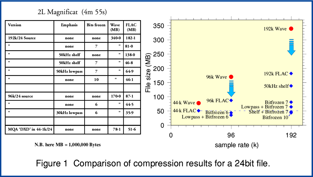
Figure 1 is an illustrative example of the processes that become relevant when we want to explore how efficiently we may be able to compress an audio file whilst retaining audio information. The values shown are for one of the demo/test files that the‘2L’ music company have made available from their website for people to try out their recordings. Here I have chosen the Arnesen Magnificat as the basis for illustrating how to reduce file (and thus also internet stream) sizes once methods like FLAC are a part of the available toolkit.
Three of the items included in Figure 1 are files downloaded from the 2L site. These initial ‘source’ files are:
Looking at these we see a fairly familiar pattern in that the 192k/24 FLAC file is about twice the size of the 96k/24 FLAC. This seems so common that it may pass without really being thought strange. But when we think about it we realise that – statistically speaking – audio details tend to be rather thinner on the ground above about 50kHz than below 20kHz. So if FLAC is working efficiently, why is the 192k version not rather less than double the size of the 96k version? OK, we’d expect it to be bigger, but why so much bigger? The factor of two seems suspect if the content is music. For Wave LPCM this would be normal as that makes no attempt to data compress. So that may lull us into accepting the same behaviour from FLAC. But FLAC compresses audio information very efficiently.
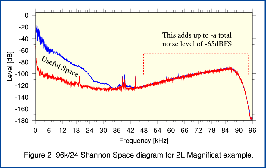
Figure 2 reveals the answer. This shows two spectra of sections of the 192k/24 recording. The red line is the spectrum of the first 0·7 sec or so. At this point the input level was wound down so the spectrum mainly shows the ‘noise level’ of the recording system including the ADC (Analog to Digital Convertor) and any following processing or downsampling 2L employed to generate the file. The blue line shows a spectrum taken for a portion of the recording where the levels of music were high. (Starting roughly 2 m 30 sec into the file.)
A 24bit LPCM recording requires a minimum total noise level for ‘dither’ purposes of around -144dBFS. Here the spectra were measured dividing the frequency range into 4096 sections. That means that if this minimal dither noise had a uniform power spectral density its level would be at around -180dBFS in each spectral section. So the total Shannon Space theoretically available for the 192k/24 bit LPCM is 180dB high and 96k wide. By choosing these values for the displayed graph we can arrange that the required number of bits per second to convey data or information will be roughly proportional to the relevant areas on the graph. This makes the graph a convenient way to get an impression, by eye, where the bits are going!
You can see that, on average, the music contributes almost nothing to what is present above about 45 kHz. In effect the useful ‘space’ taken up by the music is the area in between the red and blue lines. The sloping ‘hill’ above about 45kHz is essentially entirely composed of what we can call “process noise” which put into the file by the ways in which the recording was made and then put into the 192k file. It isn’t a part of the actual music. (And in effect, nor is the area under the red line at frequencies below 45kHz.)
Engineers familiar with digital audio will know that some ‘noise’ is actually necessary to make good digital recordings. Indeed, if none is naturally available it is routine to add this by artificial means when using an ADC to capture audio. This deliberately added noise is usually called ‘dither’. This needs to be able to ‘randomise’ to some extent the least significant bit when making recordings. The above recording is 24bit LPCM. That requires dither/noise to be provided to the ADC at a level that is around –144 dBFS. i.e. well below most music. However if we add up all the noise in above spectrum that is above about 45kHz we get a total noise level of around -65dBFS. This is around 80dB bigger than necessary! In effect, it isn’t randomising just the least significant bit of each sample value. It is randomising the smallest 12 or 13 bits of each sample! In effect, around half of all the bits being stored are randomised by overly-specified noise!
It is also possible to use Shannon’s Equation to calculate the actual number of bits per second being used to convey audio details because this is represented by the area between the two curves in Figure 2. The result comes out to about 360 thousand bits per second for each stereo channel. If this were replicated during the entire recording it would require a minimum file size of around 26 million bytes. However in practice I chose to calculate the spectra shown in Figure 2 for a section of the file where the music was loud and complex. So in reality if the analysis were to be done taking into account that quieter simpler sections contain less in the way of musical information (in Information Theory terms) this estimate of the minimum file size required would almost certainly be lower than 26 million bytes. So we can conclude that the real musical information content of the 192k file is far less than the 182 million bytes of the supplied 192k/24 FLAC file. In essence this tells us that the downloaded 192k/24 FLAC file may be more than seven times as big as theoretically necessary!
Unfortunately, “lossless” compression systems like FLAC, ALAC, etc can’t efficiently compress random noise. They have to look for ‘patterns’ in order to find ways to use fewer bits to represent the audio information. Noise lacks patterns. So FLAC struggles to reduce the number of bits required because we’re insisting that every last bit has to be preserved so we can recover it again when playing the music.
This explains the curious result where the 192k/24 FLAC file is about double the size of the 96k/24 FLAC file. The 192k file is essentially ‘bloated’ by the high levels of high frequency noise. In practice, of course, when we play the file we don’t hear this noise. Its level is still modest compared with the music, and it is well above the frequency range where our ears are sensitive. But the FLAC file still has to store all the details of the noise. The problem is that FLAC’s ability to compress is being swamped by a sea of unwanted extra noise bits.
Conceptually, the simplest and most obvious way to deal with this unwanted ultrasonic noise is to apply a filter of some kind to reduce its level before we FLAC the result. If you look again at Figure 1 you can see examples of using this approach. There I applied two different types of ‘emphasis’ filters before flaccing the results.
Figure 1 shows that if we do this and FLAC the result, we get a noticeably smaller FLAC file. This is because we have reduce the number of bits-worth of random noise that FLAC is being forced to store along with the music we want.
Note that in general if we have carefully defined the filter used before applying FLAC it will then be possible to apply a ‘correction’ filter when you want to play the resulting file. (e.g. ‘sox’ can be used with ‘treble 40 50k 1·0’ to recover the original spectrum.) This use of a ‘correctable’ filter is a method that MQA ‘origami’ also employs. But note that here we are not also ‘folding’ the information. (Nor downsampling to a lower rate.) That means we don’t have to worry about ‘aliases’ generated by the folding and unfolding when choosing suitable filters. Having made an appropriate choice we can simply employ a ‘correction’ filter that recovers the original spectral shape. The ‘treble shelf’ form of filter is particularly convenient for this sort of use.
From the above we can see that simply applying a correctable filter can allow us to slim down the size of a resulting FLAC file by reducing the impact of an unwanted and excessive amount of processing noise in the ultrasonic region. However there is an alternative approach which is simpler and has a more direct aim. This is a method I’ll call “bit freezing”. If you look again at Figure 1 you can see some examples of the use of this technique. The results show that it can have a quite dramatic effect on the size of the file when you then FLAC the ‘bitfrozen’ data.
An analogy here is a situation that sometimes crops up when someone uses a hand calculator or computer program to do a simple calculation. They might start off with some values they only know with an accuracy of say, 10%. But then do the maths and get a value displayed to, say, twelve decimals. However, having a result displayed that ‘precisely’ doesn’t mean the result is accurate to twelve decimals as a realistic value. Many of the least significant digital are essentially ‘noise’ added by trying to over-specify the result.
Similarly, a recorded file being given to you that represents the samples as 24 bit values doesn’t ensure every bit is telling you the precision of the actual wanted value. A 24 bit value may not represent genuine 24 bit accuracy. The least significant bits may be submerged in a sea of process noise. This means you can choose to ignore some of them without losing any of the genuine information about the actual audio. That said, in digital systems we tend to want to keep the ‘top’ bit or two of ‘noise’ to ensure the result is dithered because this does have some usefulness. However the lower bits are largely excess baggage. Given that they also give processes like FLAC a headache, and cause compressed files to be bloated, the logical response is to simply get rid of them. This approach aims straight at the heart of what tends to make ‘high rez’ files so large. The real problem here is often the over-specified noise, not the amount of real audio information.
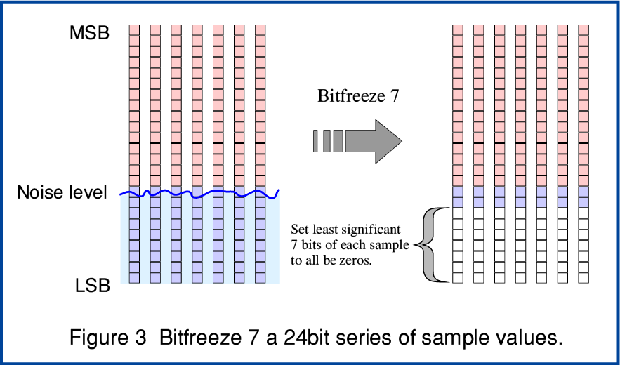
Figure 3 illustrates this process. Here we have a series of 24bit LPCM values. However in this example the recording process noise level is randomising the least significant nine bits of every sample. (i.e. the digital recording and processing system has a noise level just over -90dBFS.)
The bit freezing process essentially simply sets the lowest bits of each and every sample to ‘0’. That removes all the randomised variations in these bits and allows FLAC and other compression systems to recognise the pattern “these bits are all zeros”. So the resulting file when you FLAC the series of samples becomes significantly smaller. All we have lost is over-specified noise. In the example I’ve shown in Figure 3 I have simply frozen the lowest 7 bits of each sample, although the input random noise level submerged the lowest 9 bits. So I left in a couple of bits per sample of noise. From this you can see that the choice of how many bits you can freeze will depend on the wideband process’s total noise level. If you want to freeze as much noise as possible it is advisable to also employ a Noise Shaping technique to help ensure any real signal variations will be carried over and not ‘lost’.
Looking back again at Figure 1 you can see some examples of bit freezing the least 6 or 7 bits of the files, and the dramatic effect that has on the size required for the resulting FLAC file. In the case of the Magnificat example more than 10 bits could have been frozen because the process noise level was around -65dBFS which means distinctly more than 10 bits per sample are submerged in the noise sea! Hence in this case I was also able to bit freeze 10 bits per sample and reduce the file size by a factor of about four! However in practice in such cases it may be more convenient to just prefer to store the audio as a 16bit file anyway. Provided the requantisation was done carefully that will do the job and will have largely discarded the lowest 8 bits or so of noise so far as FLAC is concerned.
These results may seem strange at first sight. It is natural to think that ‘high resolution’ must require many bits per sample. But note that – unlike MQA – the file size reductions here do not require any change in the sample rate. The files can remain 192k or 96k sample rate, and keep their full bandwidth and time resolution with no risk of added ‘aliases’. In addition, if an emphasis filter is used, one that is fairly ‘lazy’ can be chosen and this will help ‘apodise’ the result even if you don’t then bother to correct the filter upon replay.
Note that freezing bits which are under the top bit or so of noise doesn’t significantly reduce the audio noise level when the file is played. All we have done is altered the individual noise contributions slightly, sample by sample, leaving their top bits essentially the same. Bit freezing ‘hollows out’ the needless submerged sea of bit variations that cause problems for FLAC, but still should leave enough ‘surface’ noise to avoid changing the audible results.
In some ways, the situation here has some parallels with SACD. There a series of one-bit samples are taken at a high sample rate. Yet when replayed the result has an audio resolution which exceeds the 16bits per sample of ye olde Audio CD. It can also be replaying using a ‘lazy’ filter shape that reduces the ultrasonic ‘noise’ levels. Given a high enough sample rate you don’t have to use a large number of bits per sample.
Conceptually, the problem here tends to be that it is easy for people to confuse ‘data’ with ‘information’. However although we require data to convey/store information, not all data is informative, and the container is not the contained! In the cases above quite a lot of the data is actually extra noise which is more a hindrance than a help. So when we compare a 192k/24 LPCM recording with a 96k/16 version they might actually contain almost the same information, but the 96k/16 version has lost a lot of unneeded data (noise) that can bother processes like FLAC!
From the above you should be able to see that – in terms of reducing the sizes of FLAC downloads or streams – methods like bit freezing and emphasis may be able to match or beat MQA. They also have the advantages of being ‘open’ and ‘free’. i.e. anyone can write programs to bitfreeze audio files or employ correctable emphasis. And the resulting FLAC files can be played normally.
The above shows that we should be able to employ slimmed down FLAC files or streams to obtain or store high resolution audio without any significant loss of audio details. This is potentially good news for providers as well as users because it can save them storage space and let them make more efficient use of their internet bandwidth. And without any need to reduce the sample rate or audio bandwidth. Given that, statistically, very little musical information is high in the ultrasonic region we can expect an efficient combination of the methods I’ve described to mean that even sample rates above 192k can be stored and transmitted efficiently.
However there are some special cases where can’t make use of FLAC for what the MQA patents call ‘legacy’ reasons. So let’s now look briefly at those...
Special Cases
The main special case here is if we want to be able to add to Audio CD’s a way to carry audio with a wider bandwidth. The MQA Patents propose bit stacking for this purpose. The idea being that the results should also be ‘compatible’ with ‘legacy’ players which don’t understand the MQA bitstacking and treat the results as being 16 bit LPCM.
There is, here, something of a semantic question over the meaning of terms like ‘compatible’. In some ways this MQA approach does remind me of ye olde HDCD (which stands for High Definition Compatible Disc, not Compact Disc). That also ‘hijacked’ the least significant bit to act as a data channel for non-LPCM information and then ‘scrambled’ this to make it behave like ‘noise’ when played with a system that didn’t understand HDCD encoding. Alas, HDCD was in some cases used in ways that its inventors did not intend, and the results sometimes degraded normal replay. So one concern here is that such systems can end up being misused despite the best plans and intentions of the inventors. However here I’ll assume that any MQA encoded CD is well produced with suitable care.
There is another similar question over calling an MQA’d disc an ‘Audio CD’. As with the term ‘compatible’ this depends what you mean, and possibly not everyone will take these terms to have the same meaning. In terms of the original Philips/Sony definitions of ‘Audio CD’ as laid out in the official ‘Red Book’ standards they issued, the information on such discs has to be in a 16bit LPCM format. That means that each bit in a sample is one bit of a 16bit LPCM value. Not a bitstack. However again, MQA seeks to ensure that the result will play acceptably well in a ‘legacy’ player when treated as being ‘Red Book’. The disadvantage here is that we can expect the available dynamic range, and perhaps bandwidth, when played in this way will be reduced. So those playing MQA’d CDs on ‘legacy’ equipment can expect to have smaller ‘Shannon Space’ window though which to hear the audio.
Another snag may arise for people who are now accustomed to ‘rip’ their Audio CDs to play at home using a computer system, media server, etc. The MQA system tries to employ the bottom bits of the bitstacks as efficiently as possible to squeeze in as much HF detail as it can into the smallest number of bits. It also tries to make the results seem like ‘random noise’ when treated as being part of 16bit LPCM. Given what was previously discussed about FLAC it follows from this that these ‘noisy’ bits won’t compress efficiently when we employ FLAC. So one result here is that ripped and flacced files may be larger. And since this isn’t random noise, if we employ bit freezing the HF info would be lost.
If someone is using a system that can detect and decode MQA bitstacks, they may be happy to accept that the files might be bigger than for a standard Audio CD version. Although this then does raise the question, might the file have been smaller still if the data had simply been left at a higher rate and bitfrozen as appropriate? Indeed, might that have also given more HF details because it wouldn’t have had to be squeezed into the bottom of the 16bit bitstacks? At present I can’t answer any of the above questions because we don’t know all the relevant details of MQA. All I can do is raise them for people to consider.
However, again, there may be alternatives which avoid the above potential problems and which – as with bit freezing – are free and open for anyone to use.
For example, you may already have some CDs that play happily as full 16bit LPCM discs in Audio CD players, but which present as a ‘computer’ CD when inserted into a computer’s optical drive. These are examples of other official ‘Book’ standard for CDs which essentially allow the disc to have the equivalent of ‘partitions’ for different purposes. For example: If you bought any of the re-mastered Beatles CDs that were issued some years ago you may know that each CD also included a short video clip you could watch if you loaded the disc into your computer. This is a standard facility that is now widely available. Add to this the observation that many Audio CDs containing much less than 80 mins worth of music when played. This potentially leaves space for other information.
The prospect here is that CDs could be made such that they conform with the existing standards for Audio CD and when played as such give the full 16bit LPCM. No bitstacks or data hidden in the bits given to ‘legacy’ players. But the disc could also have another partition/section with extra data placed there. This won’t be noticed by ‘legacy’ Audio CDs players. But could be read by systems like computers that can read the existing relevant ‘book’ standards.
This additional data could then provide extra audio details – e.g. a FLAC version of an 88·2k rate file containing HF data missing from the ‘Audio CD’ portion of the disc. A suitable player or computer program could read the two parts of the CD and recombine the information to get full 88.2k rate replay. Such a disc means that the only ‘sacrifice’ for users is that the Audio CD’s maximum playing duration would have to be lower than the current 80 mins or so. But given FLAC and the reality that – relatively speaking – the musical information gets sparser above about 20-30kHz this might not reduce the maximum playing time to the point which would affect most releases of high audio quality music. And this disc would be compatible in the complete sense that ‘legacy’ players get 16bit LPCM identical to what they’d have been given on a standard audio disc.
Note that I am not proposing the above as a system everyone should rush out and adopt. I am describing it simply to illustrate that there may be alternatives people might prefer to MQA. The point here is that alternatives are possible, and might be preferable.
48k/24bit bitstacks seem more likely as a candidate for use on media like ‘Blue Ray’ (BD) discs as it seems standard for BD’s of music to have a 48k/24 LPCM stereo track. In this case the bitstacks could easily leave the top 16bits for LPCM which means that it is unlikely that most people would notice the ‘loss’ of the least significant bits if they are happy with Audio CD. However given the sheer data capacity of a BD I do wonder it is simpler to just add a 96k/24 track anyway if people want a wider audio bandwidth and narrower time resolution.
All being well, I’ll deal with other aspects of MQA on another webpage...
4500 Words
Jim Lesurf
23rd Jun 2016