Getting audio into better shape
It tends to be assumed in Hi-Fi circles that ‘high resolution’ audio requires that a digital recording must have rather more than 16 bits per sample, and that 16 bits per sample simply isn’t sufficient and inevitably means ‘lo rez’. As a result, 24 bits per sample seems to have become regarded as, de facto, essential. Since a high sample rate is also expected or required, this has lead to a situation where it is assumed that files or streams have to contain at least 96k sample rate, 24 bit LPCM. And the modern expectation is to go to 192k, or higher, sample rates still with 24 bits per sample.
Unfortunately, if this is transmitted or stored as plain vanilla stereo LPCM it requires high sustained streaming rates and large file sizes. For example, a 192k/24bit stream as plain LPCM would require a sustained and reliable stream rate of about 8 megabits/sec – and this is without any extra information transfer to control the process! Similarly, a plain LPCM (e.g. ‘Wave’) file of, say, 60 mins duration would take up almost 4 GB of file storage! The good news, of course, is that we can employ ‘loss-free’ audio data compression techniques like ‘FLAC’ which can reduce the required stream rates and file sizes by quite noticeable amounts. That certainly helps, but it runs into a problem when we’re dealing with real-world examples 24 bit LPCM samples.
The reality seems to be that the content of most 24bit LPCM files/streams has a rather higher noise levels than the listener might expect from the ‘24bit’ label. In practice, many of the least-significant bits in every sample are occupied by being submerged in a sea of random noise. Now if file sizes or stream rates weren’t an issue this wouldn’t matter. But that over-specified noise wastes bits and gives lossless compression systems a headache. A loss-free method like FLAC can’t distinguish between unwanted noise and wanted details of the music. It has to assume every detail in the source file has to be kept. So it faithfully keeps all the details of the noise that are meaninglessly represented by the lowest bits of every sample. The difficulty here is that random noise is almost impossible to data-compress. This then limits how much FLAC can reduce the file size or stream rate. The result is a FLACed file or stream which is much bigger than would be necessary for the actual wanted audio.
I’ve already looked at this problem on a previous webpage which examined ways to ‘bitfreeze’ these wasted bits. That showed that it was possible to use that technique to deal with the problem and make dramatic reductions in the resulting file sizes and stream rates. However, there is another way to deal with this problem. One which digital audio engineers have known about for many years, and use routinely. Here, however, we tend to run into a risk of people becoming confused as a result of what people expect and regard as ‘high resolution’. In effect, people may easily be misled by the language which has become commonly used....
It seems obvious and plain sense to say that 24bits per sample will have more ‘resolution’ than 16 bits per sample. And in principle it makes logical sense that it will be so. However it is worth stepping back and coming again at this presumption from a fresh angle to get a clearer view. The first point to stop and take into account is that digital audio information is contained or represented in terms of a series of sample values. In effect, the information about the waveforms is distributed across a sequence of values.
So far, so obvious. But now consider things like the SACD / DSD system which actually only uses one bit per sample. Yet DSD is generally accepted as ‘high resolution’! Similarly, many modern ADCs and DACs are ‘low bit’ and represent or process the audio as a series of sample values which actually employ far fewer than 16 bits per sample! These examples give us an apparent conundrum of ‘high resolution’ audio systems which may use far fewer bits per sample than an Audio CD. The reason this is possible is that SACD and these low-bit devices use higher sample rates than Audio CD. And from the viewpoint of Information Theory it is the bitrate that determines how much detailed information can be conveyed per second. Not the number of bits per sample. The trick is to make the most efficient and effective use of the chosen bitrate.
Another way to look at this is to use an analogy like looking at boxes of soapflakes or cereal on a grocery shelf. When we look at the size of the boxes on the shelf we can get an idea of how much the box is capable of containing. But in practice the boxes may actually contain rather less of the wanted soap or cereal than they could. Here the box is akin to the bitrate or file size of an LPCM stream/file. Instead of height, width, and depth, the sample rate, number of bits per sample, and number of samples determine how many bits of information an LPCM file or stream could hold. But in practice, of course, that doesn’t tell us how well filled a particular box might be, or how much space inside it might be wasted! The fact that using a system like FLAC allows us to reduce the number of bits required to hold the audio information tells us the LPCM ‘box’ wasn’t packed full in the first place.
Pushing that analogy along, we can also see that the overall shape of the box could be altered, yet be able to contain the same amount. That’s akin to doing some kind of trade-off between sample rate and sample size. Provided we don’t alter the shape ‘too much’ (which will depend on the actual contents) all that matters is that the box has to be ‘big enough’. Information Theory formally establishes via mathematical proofs that the same sorts of ideas apply to conveying and storing information – including audio. In this case we have an added problem, though: some of the contents of the box may be unwanted excess noise that ‘bulks up’ the contents with stuff we don’t need or expect. Bitfreezing represents one way to remove this unwanted padding. That lets us use a smaller box without losing any of the wanted content.
However the fact that Information Theory allows us to vary the ‘shape of the box’ raises the question: Could – say – 192k / 16bit LPCM versions deliver exactly the same audio resolution and detail as in actual real-world examples of 192k / 24bit material, and in the process reduce the number of noise bits that bloat the file size and stream rate because of over-specified noise? It turns out that the answer to this question may well be ‘yes’! And one technique for achieving this useful outcome is called ‘Noise Shaping’. It’s a technique digital audio engineers have been using for decades for various purposes. So I’ll try to outline how it works and what it may be able to offer ‘high rez’ audio...
The big barrier at this point is that to really understand Noise Shaping in detail you also need to get to grips with some particularly complex parts of the application of Digital Signal Processing to audio. This can make even dome-brains wearing white coats scratch their heads and get a cup of tea instead. But the general idea can be illustrated by some diagrams and examples.
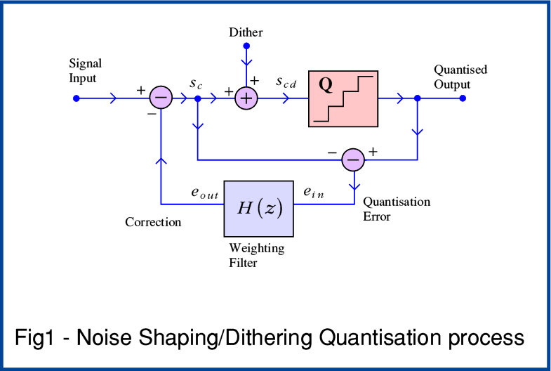
I’ll start with the arrangement shown in Figure 1, above. The signal input is, say, a stream of 24bit LPCM values arriving at a rate of, say, 192k. (I’m using these values just for the sake of example, but the same arguments would apply if I’d chosen the input to be 384k / 32 bit, or whatever.)
The central part of the system is the ‘Quantiser’ ( sometimes called the ‘Re-quantiser’) shown by the box labelled with a ‘Q’. This takes in each 24bit value and chops off the information in the least significant 8 bits. The result therefore has lost any tiny details which may have been hidden – along with a lot of the noise – in those bits. Note that just before being quantised the input has a small amount of random noise added to it. This is the ‘dither’ shown in the Figure.
It may seem odd that this process adds some noise and calls it ‘dither’. But again from Information Theory it turns out that there are good reasons to do this. And when we employ Noise Shaping, the system sets out to correct for it anyway. Again, an analogy here is perhaps to think of the way mechanical engineers generally want to remove friction from the systems they build and regard it as a bad thing. Yet screws, nut and bolts, etc only work because of the presence of friction. Similarly, there are times when some added noise actually helps.
The simplest possible quantisation system like this would do no more than add some ‘dither’ noise and quantise the result to generate a 16bit output sample from each input 24bit sample value. The dither is added to scramble away any tendency for this process to distort the result. This simple approach can easily be used, and its main drawback is that the output now has added noise which means the result has a noise level set as we’d expect to be that for 16bit LPCM.
However Noise Shaping adds a crucial process. As you can see from Figure 1 it compares the output from the quantiser with what’s being fed in before the addition of dither and the quantisation down to 16 bit. This lets it note the ‘error’ produced – i.e. it knows exactly what was ‘lost’ from that particular sample. The system then sets out to use this knowledge to re-inject the missing info by using it to alter later samples to try and ‘correct’ for the ‘loss’. In effect, this means that detailed information now need not be entirely lost. It can be used to tweak following samples to increase the faithfulness of the output series of samples and make them produce audio waveforms that are closer to the 24 bit original!
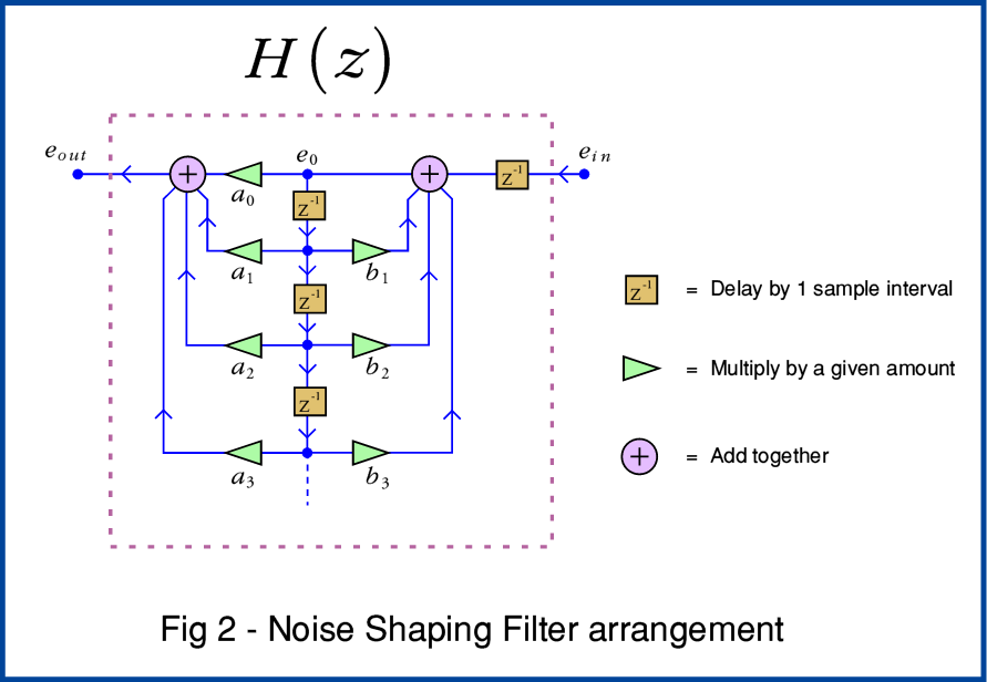
The internal details of Noise Shaping systems vary a lot. And working out the ‘best’ arrangements is a real challenge. Devising a‘Weighting Filter’ optimised for the task can be hard work. So many engineers just hunt around for and steal... erm, I mean... are inspired by a detailed design someone else has devised and published that looks like it will do the job! The general process is illustrated by Figure 2. When first seen this looks complicated, but it can be understood by starting with one of the simplest practical forms it can take.
If you look back at Figure 1 you can see that Noise Shaping is a ‘Feedback’ technique. It takes a measure of how much the output differs from the input and feeds that back as an ‘error’ value to alter the next input value. The aim being to correct or compensate for the error that was just made. In principle, this is based on the same arguments that have lead to feedback being widely used in analogue circuitry. Used well, it can improve the performance.
In a digital system the information comes as series of sample values. This error value has to be stored or ‘carried forward’ so it can be used to try and correct the next sample in the sequence. That means that the feedback path though the Filter has to include a delay. This is shown by the box with ‘z’ in it. The standard way Digital Signal Processing engineers represent a delay is to use this ‘z’-notation. The power of -1 means ‘keep the sample and pass it on after one sample interval or clock cycle has elapsed’
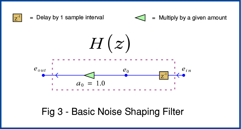
Looking now at Figure 3 we can see that this elementary Noise Shaping example simply delays the error value and then uses it to adjust the next input sample. In effect, this passes back the changes made by the quantisation and dither, and puts the info that would otherwise have been ‘lost’, into the next sample in the sequence.
The more complicated filter arrangement shown in Figure 2 uses a chain of delays and also allows the system to scale the delays. This lets much more complicated filtering processes be carried out. This can then be used to tweak or optimise the effect and get improved results. The snag is knowing just what details will provide the best results. However here for the sake of example I’ll just stick with the simplest possible example of the use of Noise Shaping, and adopt the elementary feedback filter shown in Figure 3.
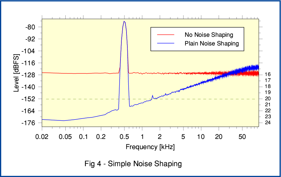
For this example the input was a 192k/24 bit LPCM stream of samples which contains a low-level sinewave at 500 Hz. I wrote a program that takes this series of values and generates two 192k/16bit versions. One generated using Noise Shaping, and one without. Figure 4 shows spectra of the results obtained by doing Fourier Transforms of the resulting 192k/16bit outputs.
The red line shows the result of just dithering (with triangular PDF dither) the quantisation to prevent systematic quantisation distortion - i.e. no noise shaping was employed. The spectrum has a white-noise background at the sort of level we’d expect for dithered 16 bit LPCM. (The total noise for properly dithered 16 bit LPCM should be around -93dBFS. However the process of calculating a spectrum divides this total into its partial contributions in each small frequency section of the spectrum. Hence the white noise level here comes out at about -128dBFS per narrow section.)
The blue line shows the spectrum for the 16bit LPCM output when the basic Noise Shaping method from Figure 3 was employed during requantisation. Here we can see that the background noise spectrum has clearly been ‘tilted’. The total noise is still at much the same level around -93dBFS. But most of the noise power is now located up in the higher frequency range above 20kHz. As a result, the output is audibly quieter, and the effective resolution is enhanced. In general, having one bit per sample more or less for LPCM can be expected to alter the minimum noise floor level by 6dB. We can also regard the effective noise level as a measure of the audible resolution. On that basis, Figure 4 shows on its right-side axis the nominal number of bits per sample required for a flat noise spectrum at that level. Looking at this we can see that the effective audible resolution will be equivalent to using between 18 and 20 bit LPCM created without noise shaping. In essence, the result should sound like 18 to 20 bit per sample LPCM despite being a series of 16bit samples. However unlike the 24bit original, the 16bit output will have lost any overly-specified noise bits which were submerged by a recording noise ‘sea’. Hence the result is not only smaller when stored and streamed as LPCM. It should also compress when FLACed to a smaller file or stream than the noise-bulked 24bit original. We’ve removed the excess fat that would have bloated FLACing.
In this elementary case the noise spectrum is just tilted in a simple manner that is far from optimum. However work by various engineers like Stan Lipshitz has shown that by appropriate filter design we can adjust the ‘shape’ of the way the noise is redistributed across the frequency range by the choice of suitably optimised filter coefficients. Doing this is quite a complex task. mathematically. So I won’t explore it beyond pointing out that if this is done we can expect to get somewhat better results – in terms of audible resolution – than demonstrated by the above very basic example. In particularly, the noise shaping can concentrate on reducing the noise in the region between 1 and 5 kHz where the human ear is most sensitive. Given this, we can expect to achieve effective resolutions equivalent to using over 20 bits per sample, despite actually having the output as 192k/16 rather than 192k/24. And since the process isn’t reducing the sample rate, it can preserve the HF details associated with the music. Indeed, if we were using 384k sample rate, the Noise Shaping could probably produce an even larger improvement when used to generate a well-shaped 16bit version!
FWIW Noise Shaping has been routinely used in professional audio. For example, Sony some years ago publicised their “Super Bit Mapping” system which was claimed to provide a resolution akin to somewhere between 18 and 20 bits per sample for Audio CD despite the CD data being 16bit per sample.
Of course, the total amount of noise isn’t actually reduced by Noise Shaping the quantisation process. The noise is, instead, shuffled around to put most of it up into the high frequency region well above 20 kHz. (This is why SACD also works, essentially by using the same trick. It is only a one-bit per sample system, yet it can give a higher resolution than 16bit LPCM in the audio range as a consequence of its Noise Shaping.) Systems which try to noise shape into low sample rates like 44.1k for Audio CD mean that the high frequency noise ’hill’ is limited to being below 22kHz. Whereas if we output sample rates at or above 96kHz we can hope to shape the noise into the region well above 20kHz and do a better job of hiding it from being audible. (Again, this is what SACD essentially does.)
As has already been discussed elsewhere (e.g. see link to bitfreezing) in general high sample rate 24 bit LPCM audio recordings tend to have many of their least significant bits drowned under a ‘sea of noise bits’. These excessively specify the random noise. Because loss-free audio compression methods like FLAC have to preserve every detail of the LPCM to allow for bit-perfect recovery they have to keep these useless extra noise details. Since random noise doesn’t compress well, this bloats the sizes of high resolution streams and files. One potential solution is to zero all the lower bits which are ‘under the surface of the noise sea’. That then allows FLAC to generate smaller files and streams which still have all the musical details. However the above shows that, in practice, an alternative method can be to carefully Noise Shape high rate 24 bit audio LPCM into 16 bit LPCM without changing the actual sample rate. This produces a result whose effective resolution is a better match to the actual resolution of real-world source material, and which can be streamed or stored more efficiently.
In engineering terms, this is a simple, free, open, and accessible method anyone can employ. The resulting files can be played in the usual ways and should yield the required audio resolution. The main problem, I suspect, for domestic audio enthusiasts, is a conceptual one. This is that people may have become focussed on a specific ‘meaning’ of the term ‘high resolution’ and may take for granted that this must include ‘24 bits per sample’. So the idea that a method as well established as Noise Shaping can allow 16bit LPCM to match what people assume they are getting from files or streams that say ‘24bit’ on the box may seem too good to be true. In some ways people may be being distracted by the size of the box rather than the content! However given SACD / DSD is based on one bit per sample, the above may help people to realise that having many more bits per sample isn’t, in itself, a guarantee you’ll actually get real higher resolution. And given the excess noise they can carry, needless added bits may simply clog up the system and increase cost and inconvenience. To get past this we have to distinguish the box from the real wanted content and avoid unwanted padding.
A version of the program source code used to generate the above results is available as NSDemo.c. I've added comments to it in case it helps. But I'm not a very good programmer! So apologies for the poor coding. If it is useful as a demo, you're welcome to write something better and then use/distribute that as you wish.
Jim Lesurf
3300 Words
9th Feb 2017