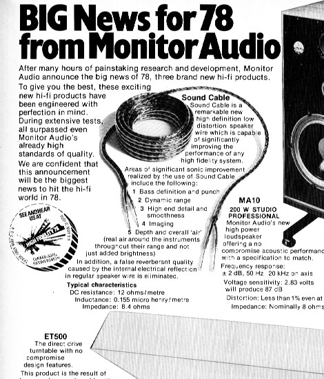
These days we’re familiar with audio magazines including adverts for a wide variety of types of ‘audiophile’ cables. But this wasn’t always the case. The first signs of the idea that loudspeaker cables mattered began to surface in UK magazines during the late 1970s. In the March and April 1978 issues of Hi Fi News there were reports of one of the first commercial ‘supercables’ to be sold on the basis that it gave superior sound. Initially, this was to be imported from Japan by Transonic Imports Limited. However that plan was swiftly overtaken by events and the cable was imported and sold by Monitor Audio. At the time it was claimed to deliver better results as a consequence of being designed to have a cable impedance of around 8 Ohms. Thus – allegedly – being a better ‘match’ for typical loudspeakers.
Subjective reviews appeared in some magazines supporting the idea that using the new cable did produce an audible improvement. But Hi Fi News was more cautious. As were members of the UK section of the Audio Engineering Society.
During 1978 a number of prominent audio engineers, including Bob Stuart, James Moir, and Peter Baxandall came together at an AES meeting to discuss cables. Having investigated the claims they were fairly sceptical. Yet now the idea that cables affect the sound is routinely accepted in the audio magazines. Adverts present all kinds of technical claims said to make each new design better than its competitors – albeit often at a price! And some magazines routinely review cables.
Alas, a lot of the apparently technical statements in adverts can be hard to decipher. To an engineer, some look suspiciously like technobabble designed to impress the innocent into opening their wallets and saying, “Help yourself!” So can we delve into the behaviour of cables and find some simple rules to guide us with assessing the claims? In particular, does the concept of cable impedance help?...
Cables are used to convey energy and information from place to place. Since the transfer is electromagnetic this means they have to ‘guide’ an EM field from the source to the destination. Ideally, we’d like the cable to have no losses, so lets start by assuming we can neglect any resistance in the cable. In a perfect world we might also wish cables had no capacitance or inductance. Unfortunately unless we use cables of zero length this isn’t possible. In our universe the cable has to have some inductance and capacitance per length. This is required to allow the cable to carry signals using the electric and magnetic fields associated with the voltages and currents.
If we study the physics of transmission lines and EM fields we find that the nominal velocity with which cables can carry energy or information is also determined by these values. Einstein’s Relativity tells us that we can’t transmit faster than ‘c’, the speed of light in a vacuum. This affects how much capacitance and inductance each metre of cable must possess. Specifically, if we take the values for the capacitance and inductance per metre for a cable and multiply these two numbers together we get a result which can’t be smaller than a given amount.
The blue line in Figure 1 shows the values of cable inductance and capacitance per metre that would allow the signals to move at ‘c’ – i.e. as fast as possible. In our universe we can choose, say, a given cable capacitance per length, but we then have to accept an inductance per length which places the cable on or above the blue line. So, for example, if we have a cable with a capacitance of 100 pF per metre, then its inductance has to be just over 0·1 microfarads per meter, or more. Not less. You may sometimes read blurb about cables that makes a highlight of the cable being ‘low capacitance’ or ‘low inductance’. But you can’t actually make both of these values ‘low’ at the same time if that would take you below the blue line. Any cable claimed to do so must come from an alternative universe, or from the set of a Star Trek movie where ‘warp speeds’ are routine engineering!
Figure 1
Larger inductances for a given capacitance are a sign that the nominal velocity with which EM fields are guided by the cable is lower than ‘c’. For the sake of illustration, the broken red line in Figure 1 indicates the combinations of capacitance and inductance which we’d get for a wave velocity of 80% of ‘c’. It also shows measured values for various loudspeaker cables. The red square shows a measurement made by James Moir and published in Hi Fi News in 1979[1]. The green circles are taken from a survey of loudspeaker cables produced by Martin Colloms published in Hi Fi News in 1990[2] As you can see, the measured results all sit above the blue line, telling us that in every case the EM field propagation velocity is somewhat slower than ‘c’. None of the cables seem to use warp engines or dilithium crystals.
The first conclusion we can find from looking at the physics is, therefore, that you should treat any claims that a cable has both ‘low capacitance’ and ‘low inductance’ with caution. The best such a cable can do is reach down to the blue line in Figure 1. That said, one curious trend shown by the results plotted in Figure 1 is that low inductance cables tend to have capacitances rather higher than the minimum allowed. There seems to be a tendency for the methods cable designers adopt to obtain ‘low inductance’ to cause an excess rise in capacitance.
Figure 2
Figure 2 uses the same measurements as Figure 1, but this time plotted to show the ‘characteristic impedance’ and signal velocities for each cable. Characteristic impedance (sometimes called surge impedance) is a property familiar to RF and communications engineers. In effect, it represents the relationship between the electric and magnetic fields that a given cable geometry uses to convey the signal[3]. The values plotted were worked out from the inductance and capacitance of each cable as that is the standard method when losses are negligible. Engineers often deliberately arranged for ‘matched’ systems where the output impedance of the source, the characteristic impedance of the cables, and the load impedance all share the same value. This can give optimum results for many situations. Looking at Figure 2 we can see two interesting trends. Firstly, almost all of the cables have nominal characteristic impedances well above 8 Ohms. (The vertical broken blue line shows where 8 Ohms crops up on the graph.) Secondly, the propagation velocities are well below ‘c’ – typically only around 50% of that value!
The red square in Figures 1 and 2 represents the original Monitor Audio type of loudspeaker cable. This was interwoven to provide a nominal cable impedance of around 8 Ohms to be a closer match for typical loudspeaker impedances. However the idea that this should produce better results is dubious for various reasons.
Firstly, most real-world loudspeakers have an impedance that varies wildly with frequency. To really match this we’d have to use a cable whose impedance also varied in the same way. Secondly, for matched operation we’d also require the amplifier’s output impedance to vary with frequency in exactly the same way. This would mean that every loudspeaker would require its own design of cable and amplifier! Fortunately, the reality is that domestic audio simply doesn’t use a matched transmission arrangement for the link between amplifier and speaker. The established standard is that the amplifier acts as a voltage source which asserts the required sound pressure variations as the same pattern of voltage variations. It then sets out to supply whatever current the speaker demands to respond to this voltage pattern. Loudspeakers are designed to respond on this basis. This approach makes no attempt to ‘match’ the impedances. Indeed, the ideal it approaches is an amplifier source impedance of zero ohms (infinite damping factor) and a cable with as near zero series resistance, etc., as possible. So it is inappropriate to assume we need an ‘impedance matched’ cable as RF and microwave engineers would use the term.
Figure 3
In addition to the above there is a third reason why attempts to match impedances are likely to prove futile. Figure 2 assumed we could ignore cable losses. But what happens when we take them into account? Figure 3 uses the same measured examples as before. However this time the analysis included the effects of factors like the resistance of the cables. You can see that once this is done the properties of the cables become highly frequency dependent! (Here I’ve only plotted 15 examples to avoid the lines merging and the graphs becoming unreadable.) At high audio frequencies the values for each cable’s impedance and signal velocity approach the results obtained by ignoring the losses. But as we drop down to lower frequencies each cable shows a tendency for its impedance to rise, and the signal velocity to fall. These variations in impedance make it even more impractical to try and obtain a matched amplifier-cable-speaker system.
I’ve highlighted the behaviour of the ‘8 Ohm’ cable measured by James Moir with a series of red squares. Its actual cable impedance is considerably higher than 8 Ohms over much of the audio band. Also, to get the claimed impedance the cable was made with a construction that produced a very high amount of capacitance per meter (around 1500pF). Unfortunately, high capacitance can cause instability with some power amplifier designs, sometimes prompting oscillations at ultrasonic frequencies. This can degrade performance or even damage the amplifier. It was reported at the time that cables of this type lead to problems with at least one commercial amplifier design of the period which I won’t Naim...
At first sight, the signal velocity results displayed in Figure 3 look quite alarming. The variations across the audio band might well worry people that these cables must ‘smear out’ the timing of complex musical signals so that the bass and treble arrive at audibly different times. Indeed, they might prompt hyperactivity amongst cable makers, trying to offer new cables they can claim will reduce these apparently undesirable effects. Fortunately all is not as the above seems...
Figure 4
Figure 4 shows the EM propagation delay times for 5 metre lengths of the same cables as Figure 3. This assumes we do have a (semi-mythical for domestic audio) matched system which means that in each case we designed the amplifier and speaker to have the same impedance profile as the cable! The plots do clearly show that low frequency signals take longer to go from amplifier to speaker than high frequencies. They also show no particular advantage in this respect for the cable that nominally had an ‘8 Ohm’ impedance. However note the units of the vertical scale. Sound travels though air with a velocity of about 340 metres/second. So in one microsecond it will travel about a third of a millimetre. This means that – if we’d carefully arranged the relevant matched situations – the ‘time smearing’ would for most cables be similar to making the sound source seem a around a tenth of a millimetre further away at low frequencies. Since normal loudspeakers (and musical instruments) are much larger than this they can be expected to introduce far larger ‘smearing’ as different parts vibrate. Also, the room reverberation will introduce reflected sounds with time delays many thousands of times greater than shown in Figure 4. Hence in normal use we can generally expect the effects like those shown in Figure 4 to be swamped by various other factors.
Figure 5
Of course, in a normal domestic setup the loudspeaker-cable-amplifier system simply isn’t matched, so the results shown in Figure 4 are inappropriate. Lets now look at a more relevant situation. Figure 5 illustrates the result we get if we use 5 metre lengths of the speaker cables, but this time we have an 8 Ohm loudspeaker load and an amplifier with a low output impedance (i.e. high damping factor). One of the graphs in Figure 5 shows the time delay produced. Looking at this you can see that the delays tend to be larger than for the ‘matched’ case. But now they are almost uniform across the audio band for most cables. The other graph displays the signal loss. This essentially shows how the sound level and frequency response are changed by using 5 metres of each of the cables rather than having the amplifier and speaker connected directly together. Some of these plots show a change in response at high frequency.
Figure 6
Figure 6 illustrates the underlaying behaviour in a clearer form, using four graphs. Each graph takes a given cable property (e.g. series resistance) and plots some aspect of behaviour against it. As before, I have assumed a 5 metre length for the loudspeaker cables, and an 8 Ohm load. The top-left graph plots the signal loss at 100 Hz versus the cable series resistance per metre. The broken red line plots what we’d get if we used a simple series resistor instead of a cable. You can clearly see that all the results sit neatly on the line. This tells us that – at low frequencies – the signal loss will simply depend on the cable’s series resistance. The top right graph plots the change in signal loss between 100 Hz and 20 kHz against the cable inductance per metre. This represents how much the frequency response droops at 20 kHz. Here the blue broken line shows what we’d get from a pure inductance. Similarly, the bottom left graph shows a plot of the signal delay at 1 kHz versus inductance. In these two cases we can see that for modest or low cable inductances the cables all sit close to the blue line. The final (bottom right) graph plots the signal delay against the cable impedance at 1 kHz. On this graph, although most of the points for the various cables do cluster together, they don’t tend to sit neatly on a line to the same extent as in the other graphs.
The main conclusion we can draw from the above results is that the nominal characteristic impedance of a domestic loudspeaker cable isn’t really a useful guide to performance. But for cables which have reasonably low series resistance and inductance, these values are good predictors of effects on the audio band frequency response, etc. Since low series resistance and inductance produce low loss and a flatter response, this is likely to be the preferred choice in many cases. So the initial point an engineer might make when choosing loudspeaker cables would be to look for low resistance and inductance. In itself, the nominal cable impedance isn’t particularly relevant. That said, low cable impedance is associated with low inductance, so going for low impedance may be sensible as it means you tend to get what may be more significant - low inductance cable. For that reason cable impedance might be of interest if a manufacturer doesn’t specify inductance. But for loudspeaker cable, it tends to be the series inductance and resistance that are of primary interest. However this isn’t the whole story, so I hope to say more about cable effects in the future.
Jim Lesurf
2600 Words
20th May 2008
[1] Loudspeaker Cables James Moir Hi Fi News pp 67-75 May 1979
[2] The Cable Survey: Part 2 Speaker Wires. M. Colloms Hi Fi News pp 50-53 July 1990
[3] If you wish to know more about this, go to the webpage at
http://www.st-andrews.ac.uk/~www_pa/Scots_Guide/audio/Analog.html
and follow the links there to ‘part 6’ and ‘part 7’.