Audio CD Quality – a health check!
How do you check just how well recorded and produced the actual audio on an Audio CD may be? Because the CD usually contains music this isn’t always easy due to the very complex and time-varying nature of many musical waveforms. However one approach is to perform some fairly basic statistical analysis. In principle, this approach can be very simple. But the snag is that it tends to involve a lot of data (sample) values to number-crunch. For example, a 5 minute long track will contain 13 230 000 sample values per channel. So even a moderately long track would tend to overwhelm most general purpose statistical applications like a desktop spreadsheet.
To tackle this, I therefore wrote a dedicated computer program program that can ‘rip’ the samples from an Audio CD track and – instead of playing them or saving them to a file – performs a statistical analysis on the values it finds. It then provides the results so you can look for any signs of problems. (My initial program only runs on RISC OS, but all being well, I’ll soon produce a Linux version, so stay tuned if you’re a Linux user!) The program reads through the sample values and counts up how often each possible value occurs. It then outputs these counts so you can see their distribution.
To show how this works I’ll use a few examples. And I’ll start with a good-quality recording so you can see what the results should look like...
Decca Sound - The Analogue Years
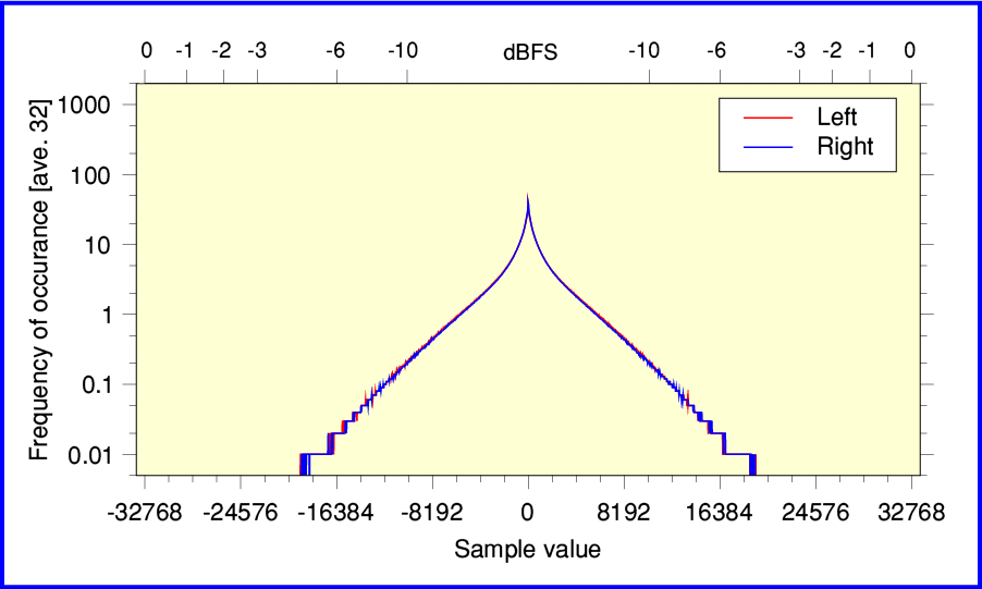
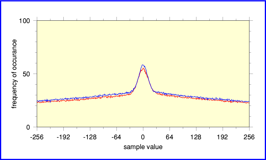
The graph plotted above shows the results for a CD taken from the recent “Decca Sound - The Analogue Years” box set of 50+ CDs. It’s actually from track 5 of disc 28, which contains recordings of Mendelssohn Symphonies played by the LSO, conducted by Abbado. As you might expect, you can see that sample values near zero occur much more often than ones near the extremes. Indeed, you can see that the samples present are all below -3dBFS, so there is no risk of clipping.
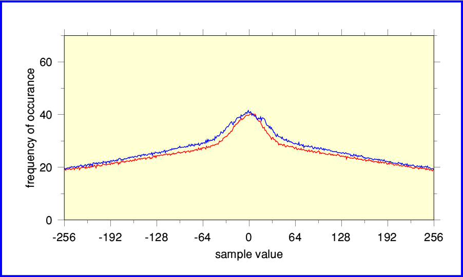
If we zoom in and just examine the near-zero value in more detail the results approximate to a the kind of general ‘bell’ or ‘hill’ shape statisticians might expect. The signs are that this recording is fine. There are no obvious problems with the way it was digitally sampled from the analogue master tape and mastered onto the CD. And, yes, it sounds good, too!
Having seen that we can move on to a ‘rogue’s gallery’ of other examples...
Jimi Hendrix -Are You Experienced (Experience Hendrix version)
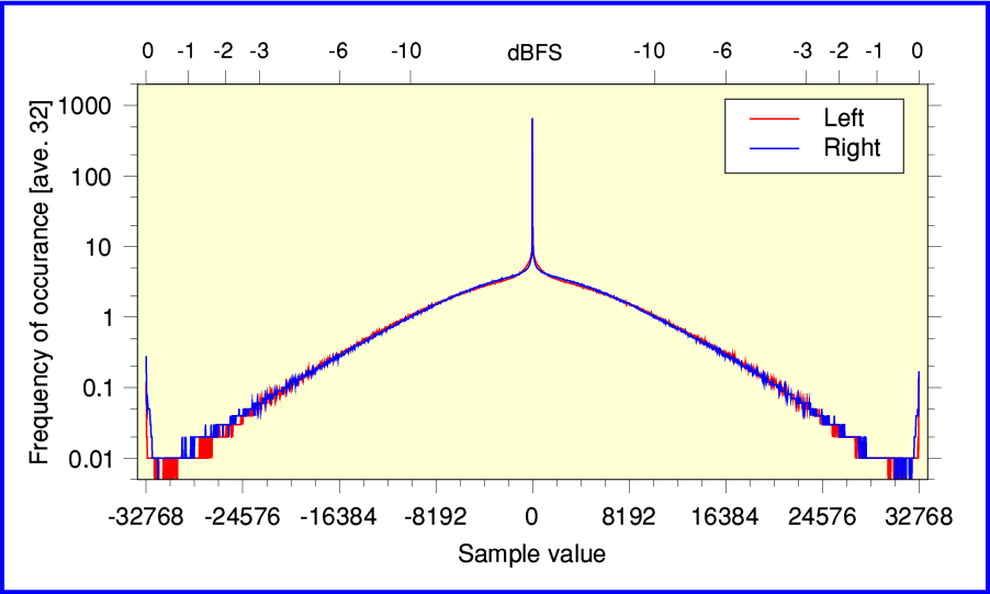
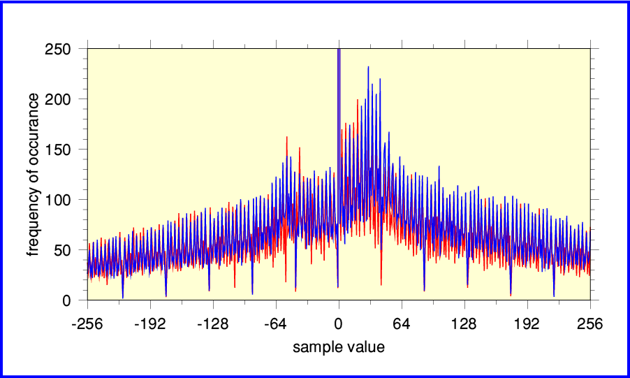
The above shows the results from the late-1990’s “Experience Hendrix” remastering of Purple Haze on MCD11608. The main feature to note here is how the shape has ‘wings’ that rise as the plots approach +/- 32768. This is a sign that the digital transfer was made with the gain set too high. The result is clipping. For some parts of the original waveform the musical peaks are requiring sample values beyond the range possible for an Audio CD. So the result will be clipping distortion as the tops and bottoms of louder parts of the musical waveforms are scissored flat! I’m afraid this kind of fault is depressingly common for pop/rock Audio CDs. If the producers making the CD from the analogue tapes had dared to turn down the level by a dB or so, the result would have sounded better. But either they had no clue, or didn’t care, and assumed LOUDER IS BETTER and to hell with faithful sound quality...
Debussy - Images for Orchestra
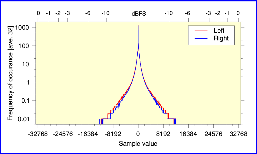
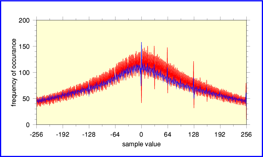
The above shows the full-spread of results for track 1 from Debussy’s “Images for Orchestra”, played by the LSO and conducted by Andre Previn. This is taken from EMI CDC 747 001 2. I think this was one of the very first classical music CDs released by EMI. The graph above looks OK although the center peak seems a little high. And the analysis program implies there was about 8 seconds of ‘Digital Black’. (The track is about 434 sec long in total.)
Digital Black is a term used to indicate a stream of successive zero-values. This is sometimes employed to add a silent lead-in or lead-out to a track. It may also occur if there was a crude edit to remove a blemish or join two sections together.
Whatever the cause, the result is that the number of samples with a value of zero is boosted and we get a central peak that sticks up well above how often sample values like +1 or -1 occur. This allows the analysis to estimate how much Digital Black has been added to the audio.
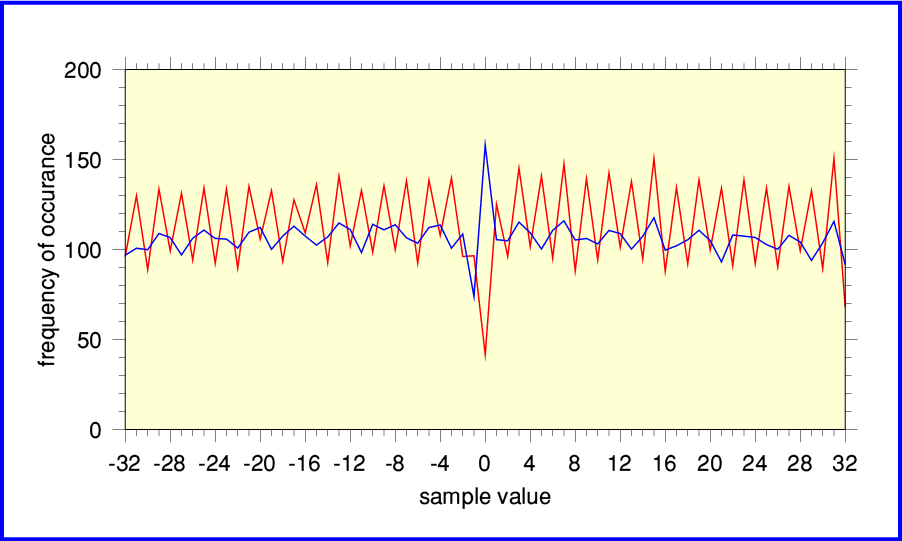
The above shows the results when we zoom in and look at the central part of the Debussy results in more detail. Now it’s fairly obvious that something is wrong. Instead of the smooth bell shape we found for the Decca CD of Mendelssohn, this distribution has ‘stalactite and stalagmite’ spikes with regular spacings. It also seems to have two side-hills at sample values around +/- 50.
Narrow dips (stalactites) occur when a sample value occurs far less often than its near-neighbours. Narrow upward spikes (stalagmites) appear when a sample value occurs far more often than its neighbours. In both cases it isn’t something you’d expect to arise naturally with ordinary acoustic or orchestral music. So these spikes act like flags, pointing to a flaw in the digital recording or processing.
Uniformly spaced spikes in the distribution can arise for various reasons. The easiest way to explain how they can arise is to consider someone deciding to adjust the sound level in order to make the music on the CD slightly louder. However they then make this adjustment poorly – possibly without realising what then happened. To illustrate this, lets imagine we wanted to make all the sample values about 20% larger. (This increases the sound level by about 1·5 dB.) The key snag here is that all the sample values on an Audio CD are integers. So when we change, say, a sample value of 7 we really want a result of 8·4. But we can’t put 8·4 onto the CD because that’s not an integer. We have to choose either 8 or 9 instead.
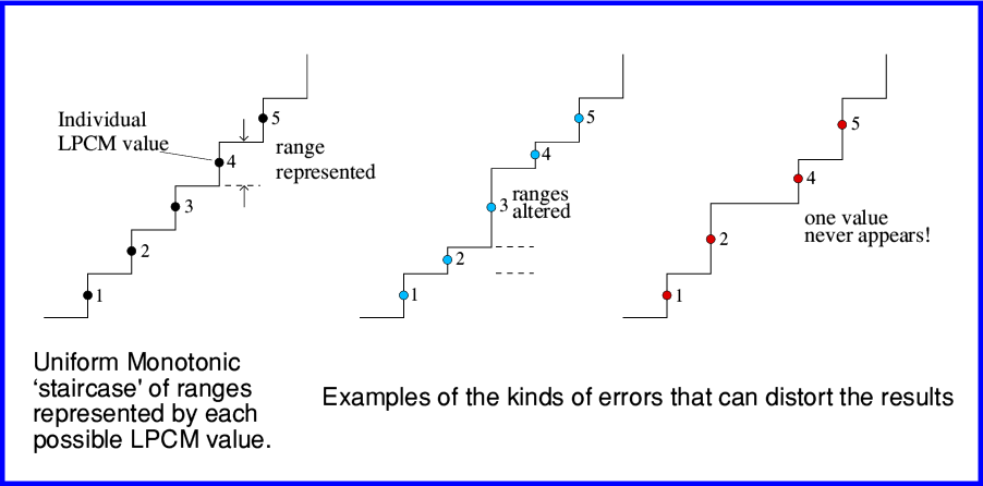
Problems of this kind are sometimes referred to as ‘Monotonicity Errors’. The theory behind LPCM is that each value represents a specific range which is part of an overall pattern of possible analogue levels. The set of possible LPCM values is required to form a neat and uniform ‘staircase’ as shown on the left in the above diagram. Note that each step has the same height, and they share out equally the full possible input range of sound levels. And the LPCM values (numbers) are in simple 1,2,3,... sequence, labelling the steps in order.
Your DAC or CD Player is designed on the basis that this is what the LPCM values represent. So when it uses them to generate an analogue waveform it has to take for granted that the series of digital values it is given accurately follow this rule. It can then know what output pattern to produce. However if some earlier link in the chain from the studio to you gets this wrong the result will be distorted.
The above diagram illustrates two of the possible ways monotonicity errors can mess up the final result. Problems with the recording process or alterations along the chain can mean that the LPCM the values you were given don’t represent a neat uniform staircase. Some values may represent a range quite different to your DAC assumes. Other values may have been ‘lost’ entirely. Either way, the result is distortion. Sadly, there are lots of ways for recording studios, etc, to mess this up. And your DAC has no way to correct the resulting errors.
Information engineers have known about this problem for decades, so it isn’t a problem from their point of view. Techniques like ‘dithering’ and ‘noise shaping’ deal with this, and have been available since before Audio CD was launched. However that doesn’t mean every record producer or remasting engineer knows about them. Nor that the equipment they use employs them. So things can – and do – go wrong. Continuing with our example, what can happen is illustrated by the table below. This just looks at a small range of the possible values in detail.
| input sample | 0 | 1 | 2 | 3 | 4 | 5 | 6 | 7 | 8 | 9 | 10 | 11 | 12 |
| x 1·2 | 0 | 1·2 | 2·4 | 3·6 | 4·8 | 6·0 | 7·2 | 8·4 | 9·6 | 10·0 | 12·0 | 13·2 | 14·4 |
| = output sample | 0 | 1 | 2 | 3 | 4 | 6 | 7 | 8 | 9 | 10 | 12 | 13 | 14 |
Because we have to output integers, no sample value in the input can ever give a ‘5’ or an ‘11’ in the output. So some sample values never occur if we make an audio file louder in this over-simple way. Some possible sample values become rarities as a result. That said, they may not vanish entirely from a plot like the above. There are various reasons for this. For example, perhaps only a part of the track examined had the gain change applied to it. We can then get some examples of the ‘excluded’ values from the portion of the track that didn’t have its volume level fiddled with in this manner. In general, dips (stalactites) can be caused by poorly done amplifications, and peaks (stalagmites) where some values occur more often than their neighbours can arise due to badly done reductions in level. And both may occur if a series of such processes were applied before the result went onto the CD.
The moral here is that professionals who ‘re-master’ material (and design the equipment) really do need to understand what actually happens when they shift a slider or rotate a knob on their control desk. Otherwise they can easily end up degrading the result without realising what they did.
Regular spikes in the sample value distribution can be caused by various types of imperfection. For example, a poor-quality Analogue to Digital Convertor (ADC) may not work correctly and produce similar effects. But whatever the cause. they are a sign that something may be wrong. How much the sound quality is affected will depend on the circumstances. As usual, the devil is in the details!
Elgar – Sea Pictures
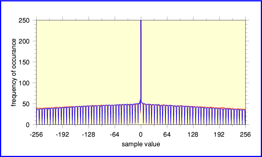
The above plot shows results for Elgar’s “Sea Pictures” (Where Corals Lie) performed by Janet Baker with John Barbirolli conducting the LSO. This is usually coupled with the du Pre / Barbirolli / LSO version of Elgar’s Cello Concerto. These recordings are among the most well-known and enduringly popular classical recordings ever made. Alas, the above results – which come from an early EMI Audio CD release (CDC 747 329 2, dated 1986) – show clear signs of some problems with the distribution of sample values.
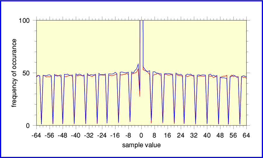
Zooming in to examine a narrower range of sample values makes the situation clearer. The pattern of stalactites implies that an alteration was made without the process being correctly dithered or noise-shaped. The result is a form of ‘grainy’ distortion. It is a shame that EMI failed to get this right given how well-loved this recording has become. Fortunately, there have now been later re-masterings that have been done with more care and skill.
The above plot shows the results for the same performance of “Where Corals Lie”. This time taken from the CD layer of a re-mastering released by EMI Virgin Classics on a dual-layer CD/SACD set 2SACD50999 in 2012. The same master tape, but evidently a far better digital version – even if you ignore the SACD layer! No sign here of any digital conversions or processing being poorly done.
Elgar Nimbus CD
The above shows the results for a Nimbus CD produced from a digital recording they made in 1983. Nimbus were one of the small companies who were early adopters of Audio CD. This example is taken from Nimbus NIM 5008 which contains Elgar string music played by the ESO, conducted by Boughton. It sounds good, but by looking at the above plot you can see that there are imperfections.
Zooming in makes the nature of those imperfections clearer. The Left channel results (shown in red) seem to regularly alternate up and down from one sample value to the next across the distribution. This is characteristic of recording with an ADC whose sampling isn't fully linear below the 15-bit range. Similarly, the Right channel (blue) levels cycle every time we move four steps up or down across the range of possible sample values. This implies a linearity which is limited below the 14-bit range. In effect, although the ADC output 16-bit values, their accuracy wasn't fully up to what theoretically should be possible for 16-bit. The effective accuracy is more like 14- or 15- bits per sample. This was actually a common problem for both early audio recording ADCs and early CD players! Alas, although you can buy a newer, better player, the effects produced by the ADC would remain.
Summary
I have only shown a few examples here to illustrate how the problems appear when you do a statistical examination and plot the results. But it seems clear that many early Audio CDs in particular show signs of problems. Alas, even some recent CDs show signs of these problems. So you may find that ones being sold even now fall into the same traps of being badly converted or processed before the results get onto the CD. Because of this, you may find it useful to run a similar ‘Health Check’ on any of your own CDs that don’t sound as good as you feel they should. And of course, downloaded digital audio files aren’t immune to such problems. To find out more about that, please have a look at the Flac Health Check webpage I have produced.
If you wish you can obtain a copy of the !CD_HealthCheck program I used to generate the above results from my software page. Versions are available for Linux and RISC OS.
Historic Footnote:
|
At the Audio Engineering Society Convention held in Paris in February 1995 a presentation was given on: Evaluation of digital systems and digital recording using real time audio data. Knee and Hawksford (University of Essex). This outlined a computer system designed to capture the spdif digital audio output stream from a suitable Audio CD player. It performed a count on the number of occurrences of each possible digital sample value of a 16 bit LPCM stereo stream. Then presented the results as Probability Density Function. The system consisted of a hardware card plugged into the ‘podule’ backplane interface of an Acorn Archimedes desktop computer. The dedicated podule hardware collected the sample values and performed the basic counts of how often each possible value occurred. The system acted as quasi-real time monitor displaying the PDF of the stream of sample values. Some examples of the resulting raw distributions where shown along with some comments about possible causes of irregularities. I don’t know if any system like this became widely used in studios, etc. The system described in 1995 lacked further steps like carrying out an FFT on the PDF to make the regularity of any patterns easier to diagnose. (See the Flac Health Check page for details of that.) It was also essentially limited to real-time 16bit audio and spdif. But it is interesting that the system doesn’t seem to have been widely adopted given that the initial results demonstrated that problems existed. |
1800 Words
Jim Lesurf
18th Apr 2015