Flac Health Check!

Having written a program that carries out a statistical examination of the audio sample values on an Audio CD I decided that the next logical step was to produce a similar program to examine Flac files. This is a bit more complicated to achieve for two reasons. Firstly, Flac files require ‘unpacking’ because the audio sample values are stored inside them in a (loss free) compressed format. Secondly, Audio CD tracks always have the same sample rate – 44,100 samples per second (44.1k) and the same bit-depth – 16 bits per sample. Whereas Flac files can have various sample rates and bit-depths. However I have now developed a program to examine stereo Flac files that use the standard rates from 44,100 to 192000 samples per second. And the program can understand both 16-bit and 24-bit samples. This means it should work with most of the flac files which Hi-Fi stereo audio enthusiasts would be interested in examining.

If you want to understand more of the details of how the analysis is done, and interpreting the results I recommend you initially read the CD Health Check webpage because the two programs essentially carry out the same analysis, and output results in much the same way. So from here on I’ll assume you’ve already read that web page and I don’t need to repeat on this page everything it explains.

To check that the two programs work in equivalent ways I initially generated some Flac files from Audio CD tracks that I’d already analysed using the CD Health Check program. This confirmed that they gave the same results, just as they should.

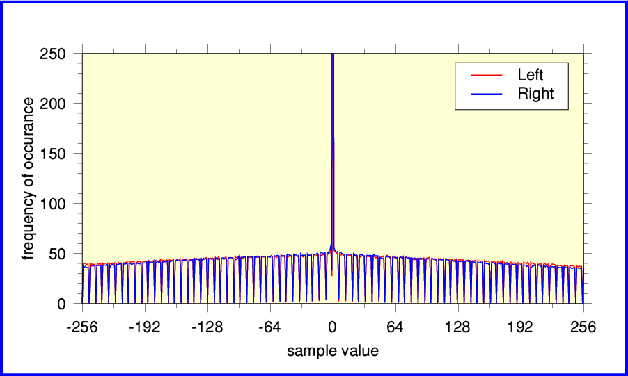
To illustrate that, Figure 1 above shows the results for a flac file generated from the same Elgar/Barbirolli ‘Sea Pictures’ CD track as I used as an example for CD Health Check. The results from the Flac file are the same as those taken directly from ripping the CD.

An alternative way to view the variations in how often each sample value occurs is to carry out a Fourier Transform of the distribution of how often each sample value occurs. In this case that gives the result shown below.

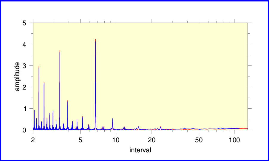
Figure 2 above shows the ‘sample interval spectrum’ of the distribution in Figure 1. In order to interpret this it’s important to be aware that this is quite different to the kinds of spectrum people normally associate with audio signals. The common practice is to do a Fourier Transform of how the sample values vary with time. That generates a frequency spectrum showing how the signal level fluctuates as time passes. However here I have Fourier Transformed the distribution of how often each possible sample value occurs if we check all the samples in the entire file (or Audio CD track).

Looking at Figure 2 we can see a clear spike at a sample interval of just under ‘7’. If we look again at Figure 1, sample values of ... -21, -14, -7, 0, 6, 13, 20, ... occur less often than their neighbouring values. The ‘rarity’ of those values which differ by about ‘7’ generate a spike at about ‘7’ in the interval spectrum. In this particular case, the oddly regular behaviour is clear in Figure 1. But in more subtle or complex cases the interval spectrum shows up features which are hard to spot in the count distribution. Indeed, you can see variations with other sample value intervals in Figure 2 which would be hard to spot from looking at Figure 1.

The above is, of course, based on 44.1k / 16-bit material, so let’s now look at two contrasting examples of 96k / 24-bit ‘high resolution’ files available commercially for downloading.

Benjamin Britten: Storm – Sea Interlude from Peter Grimes

The first 96/24 flac file example is taken from a high resolution remastered issue of the ‘Peter Grimes’ opera. This was initially recorded by Decca long before digital audio was available. The performance is a historic one conducted by Benjamin Britten. In many ways it’s an outstanding recording and performance.

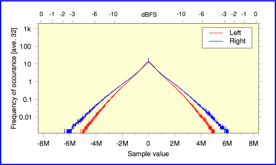
Figure 3, above shows the overall distribution of how often various sample values occur during the ‘Storm’ sea interlude’s flac file. About the only point worth mentioning is that the right-hand channel seems to reach slightly higher peak levels.

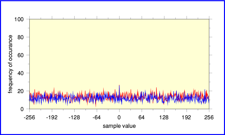
Figure 4, above, shows the central range of the distribution in more detail. Despite a small excess of zero values, there is no obvious sign of any significant problems.

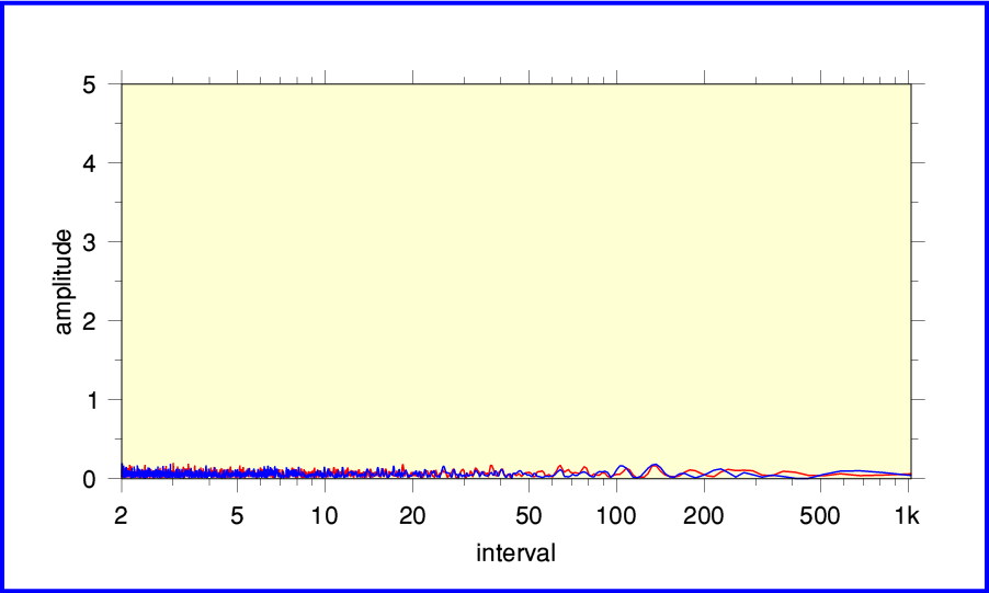
Figure 5, above, shows the interval spectrum of the distribution. This also shows no obvious sign of any flaws in the sampling or digital processing that generated the flac file. The variations displayed seem characteristic of statistical ‘noise’ caused by the finite duration of the file.

When listening to this file (and, indeed, to earlier CD and LP versions from Decca) I’ve always been impressed by the clear and natural sound quality. The above serves to confirm my impression that this 96/24 file is a very well made high resolution transfer of a superb original recording and performance.

George Harrison: My Sweet Lord – Demo early version

A year or two ago a series of demos and other alternate versions of songs by George Harrison were released on CD and as high resolution 96/24 flac files. I chose one example to examine here. The file I chose essentially consists of George Harrison singing whilst playing a guitar as a demo/test of the song.

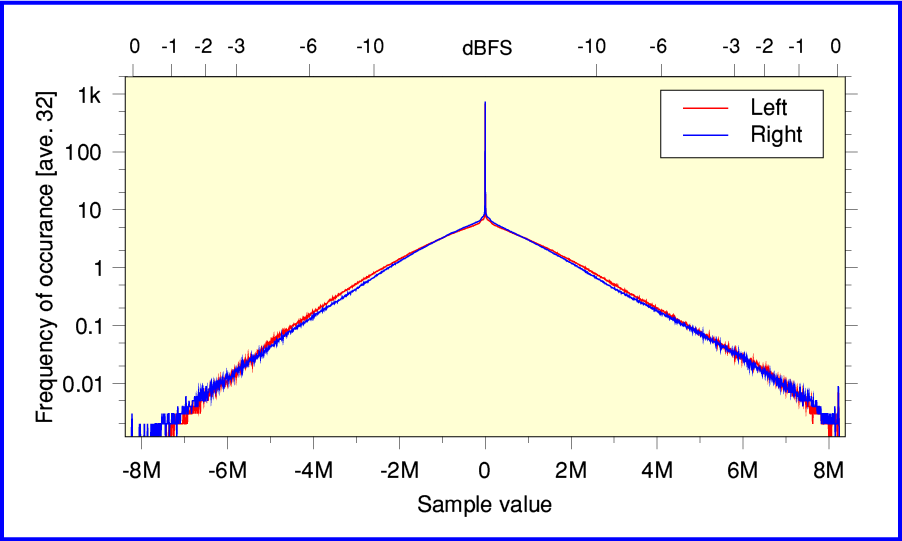
Figure 6, above, shows the overall distribution of sample values in this 24-bit file. Alas, you can see some signs of clipping due to the transfer level being too high. This is indicated by the way the distribution has small side-spikes at the ends of the distribution. This occurs because the sound waveforms were actually peaking at higher levels than could be represented at the chosen transfer gain, so those values all got scissored. This is a shame as it could have been avoided simply by using a gain that was a dB or so lower when making the transfers to digital. Upon replay this would have made very little difference to the audible loudness, but could have avoided the waveform distortions produced by clipping.

There also seems to be an oddly high zero spike. More on that below...

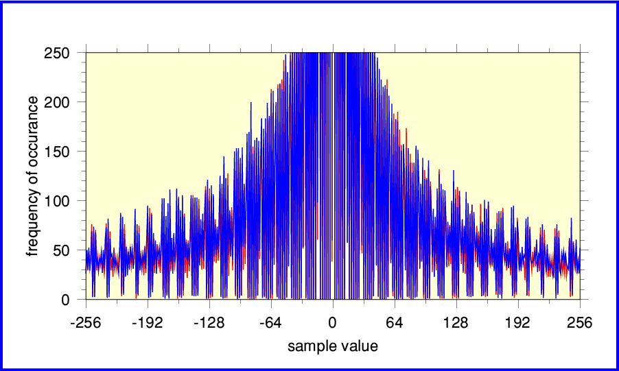
Figure 7, above, displays the central part of the distribution in more detail. This shows some signs that not all is well. It is fairly obvious that some values occur more often than others, and this varies across the distribution in a structured manner. It implies either the use of a poorer ADC than was used for the Sea Interlude example, or poor digital processing prior to creation of the flac file. The spike which seems to be at zero sample value in Figure 6 seems to actually spread across a small range of near-zero values. This is an odd effect which could occur for various reasons but may be harmless. My best guess as to the cause of the uneven distribution and spread central peak is that some kind of ‘low bit’ ADC (or SACD recording) was used along with insufficient dithering to achieve truly smooth and accurate 24-bit sampling of the released flac file.

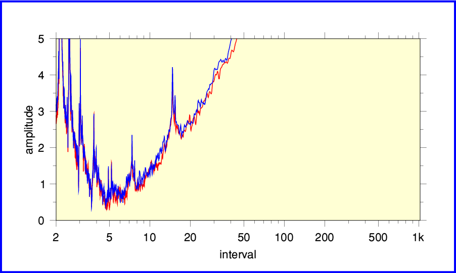
Figure 8, above, confirms that the distribution is far from being as ‘clean’ as the Sea Interlude example. The signs are that this digital remastering from the source material isn’t as good as it might be. The Sea Interlude shows that far better 24-bit transfers are possible.

Apples and Oranges? – 16-bit versus 24-bit

Given the results above its worth adding a word of caution about the interpretation of 24-bit results. If you look at Figure 8 you might assume that the Harrison 96k/24 file was as poorly done as the 16-bit Elgar Sea Pictures example shown in Figures 1 and 2. However that wouldn’t be fairly comparing like-with-like. When a range of levels is sampled with 24-bit values the samples can resolve details that are 256 times smaller than if we’d used 16-bit values. What this means is that problems which show up over sample intervals of less than 1024 in 24-bit results would be too fine to detect with a 16-bit version. In effect, 24-bit sampling is far more precise, so far smaller imperfections can be seen in the results. To illustrate this I used the ‘sox’ audio program to generate a 44.1k/16-bit downconverted version of the Harrison and then examined that.

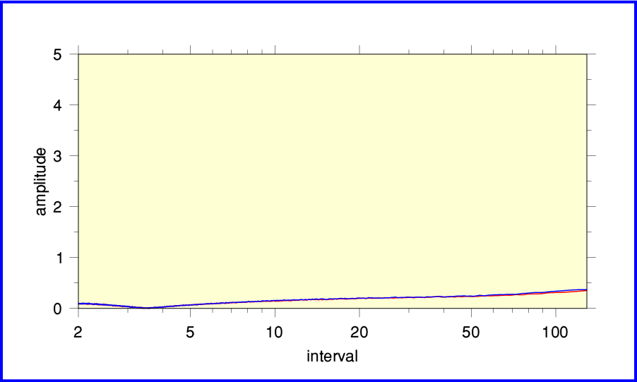
Figure 9, above, shows the resulting interval spectrum. This looks far ‘cleaner’ than the 24-bit version. The main reason for this is that a sample value interval of ‘2’ for the 16-bit version corresponds to ‘1024’ for the 24-bit version. Downcoversion has essentially smoothed away the finescale variations which were so obvious in the 24-bit results. In addition, converting the sample rate down from 96k to 44.1k smooths the results in time. That can smooth away short-term sampling flaws.

The implication is that the 24-bit flac file of My Sweet Lord may be sampled adequately for then going on to make a good Audio CD. But isn’t up to the levels of smooth and accurate sampling which 24-bit can provide when done ideally well. So the general bottom line here is that it is easier to compare files of the same sample bit-depth (and rate) than to compare files of different rates and/or bit-depths.

The good news, though, is that it is clearly possible for 96k/24 flac files to be very well produced and deliver excellent results. The Sea Interludes from Peter Grimes is a wonderful example of this.

If you wish, you can obtain a copy of the Flac_HealthCheck program I used to generate the above results from my software page. Versions of the program are available for Linux and RISC OS. The source code is provided and anyone who wishes is welcome to use this to produce versions for other operating systems.